HOME
Installation
This chapter guides you through the entire setup process required to use artemis_crib effectively. By following the steps outlined in the subchapters, you will configure all the necessary tools, environments, and directories to ensure a seamless workflow for analysis tasks.
Below is an overview of the setup process, along with links to detailed instructions for each step.
-
Ensure all required compilers, libraries, and dependencies are installed for compatibility with ROOT and artemis.
-
Set up a Python environment using tools like
uvto support pyROOT and TSrim. -
Install ROOT from source and configure it for use with artemis.
-
Clone, build, and configure artemis.
-
Set up tools for energy loss calculations, essential for analyzing experimental data.
-
Configure NFS mounts to access remote file servers or external storage.
-
Create and configure the
art_analysisdirectory, which serves as the workspace for all analysis tasks.
Requirements
This page outlines the packages required to run artemis_crib, including ROOT. Since most of the code is based on ROOT, please refer to the official ROOT dependencies for more information.
Compilers
- C++17 support is required
- gcc 8 or later is supported
- (currently Clang is not supported)
Required packages
The following is an example command to install the packages typically used on an Ubuntu-based distribution:
sudo apt install binutils cmake dpkg-dev g++ gcc libssl-dev git libx11-dev \
    libxext-dev libxft-dev libxpm-dev libtbb-dev libvdt-dev libgif-dev libyaml-cpp-dev \
    htop tmux vim emacs wget curl build-essential
- The first set of packages (e.g.,
binutils,cmake,g++) includes essential tools and libraries required to compile and run the code. libyaml-cpp-dev: A YAML parser library used for configuration and data input.htop,tmux,vim,emacs,wget,curl: Optional but commonly used tools for system monitoring, session management, and file downloads, making the environment more convenient for server-side analysis.build-essential: A meta-package that ensures essential compilation tools are installed.
To use pyROOT or the Python interface of TSrim, Python must be installed.
Although Python can be installed using a package manager like apt (sudo apt install python3 python3-pip python3-venv), it is recommended to use tools such as pyenv to create a virtual environment.
Popular tools for managing Python environments include:
If you plan to use pyROOT, ensure that the Python environment is fully set up before proceeding to the next section. Instructions for setting up the Python environment are available in the Python Setting section.
CRIB analysis machine specifications
The functionality of artemis_crib has been confirmed in the following environment:
- Ubuntu 22.04.4 (LTS)
- gcc 11.4.0
- cmake 3.22.1
- ROOT 6.30/04
- yaml-cpp 0.7
- artemis commit ID a976bb9
Python Environments (option)
By installing Python, you can use pyROOT and TSrim directly from Python. However, Python is not required to use artemis_crib, so you may skip this section if you do not plan to use Python.
Why Manage Python Environments?
Managing Python environments and dependencies is crucial to avoid compatibility issues. Some configurations may work in specific environments but fail in others due to mismatched dependencies. To address this, we recommend using tools that handle dependencies efficiently and isolate environments.
Popular Tools for Python Environment Management
| Tool | Description |
|---|---|
| pyenv | Manages multiple Python versions and switches between them on the same machine. |
| poetry | A dependency manager and build system for Python projects. |
| pipenv | Combines pip and virtualenv for managing dependencies and virtual environments. |
| mise1 | Runtime manager (e.g., Python, Node.js, Java, Go). Ideal for multi-tool projects. |
| uv | A fast Python project manager (10-100x faster than pip), unifying tools like pip, poetry, and pyenv. |
The author (okawak) uses a combination of mise and uv to manage Python environments.
If your projects involve multiple tools, such as Python and Node.js, mise is highly effective for unified management.
However, if you work exclusively with Python, uv is a simpler and more focused option.
Using uv for a Global Python Environment
This section explains how to use uv to set up a global Python environment, required for tools like pyROOT. uv typically creates project-specific virtual environments, but here we focus on configuring a global virtual environment. For other methods, refer to the respective tool's documentation.
Step 1: Install uv
Install uv using the following command:
curl -LsSf https://astral.sh/uv/install.sh | sh
Follow the instructions to complete the installation and configure your environment (e.g., adding uv to PATH).
Verify the installation:
uv --version
Step 2: Install Python using uv
Install a specific Python version:
uv python install 3.12
-
Replace
3.12with the desired Python version. -
To view available versions:
uv python list
Currently, Python installed via uv cannot be globally accessed via the python command.
This feature is expected in future releases.
For now, use uv venv to create a global virtual environment.
Step 3: Create a Global Virtual Environment
To create a global virtual environment:
cd $HOME
uv venv
This creates a .venv directory in $HOME.
Step 4: Persist the Environment Activation
Edit your shell configuration file to activate the virtual environment at startup:
vi $HOME/.zshrc
Add:
# Activate the global uv virtual environment
if [[ -d "$HOME/.venv" ]]; then
    source "$HOME/.venv/bin/activate"
fi
Apply the changes:
source $HOME/.zshrc
Verify the Python executable:
which python
Ensure the output is .venv/bin/python.
Step 5: Add Common Packages
Install commonly used Python packages into the virtual environment:
uv pip install numpy pandas
Additional information
- For more detail, refer to the uv documentation.
ROOT
The artemis and artemis_crib tools are built based on the ROOT library. Before installing these tools, you must install ROOT on your system.
Why Build ROOT from Source?
Since artemis and artemis_crib may depend on a specific version of ROOT, it is recommended to build ROOT from source rather than using a package manager. This approach ensures compatibility and access to all required features.
Steps to Build ROOT from Source
-
Navigate to the directory where you want to install ROOT:
cd /path/to/installation -
Clone the ROOT repository:
git clone https://github.com/root-project/root.git root_src -
Checkout the desired version (replace
<branch name>and<tag name>with the specific version):cd root_src git switch -c <branch name> <tag name> cd .. -
Create build and installation directories, and configure the build:
mkdir <builddir> <installdir> cd <builddir> cmake -DCMAKE_INSTALL_PREFIX=<installdir> -Dmathmore=ON ../root_src- Set
mathmoretoONbecause artemis relies on this library for advanced mathematical features.
- Set
-
Compile and install ROOT:
cmake --build . --target install -- -j4- Adjust the
-joption based on the number of CPU cores available (e.g.,-j8for 8 cores) to optimize the build process.
- Adjust the
-
Set up the ROOT environment:
source <installdir>/bin/thisroot.sh- Replace
<installdir>with the actual installation directory. - Running this command loads the necessary environment variables for ROOT.
- Replace
Persisting the Environment Setup
To avoid running the source command manually each time, add it to your shell configuration file (e.g., .zshrc or .bashrc):
echo 'source <installdir>/bin/thisroot.sh' >> ~/.zshrc
source ~/.zshrc
This ensures that the ROOT environment is automatically loaded whenever a new shell session starts.
Important Note for pyROOT Users
If you plan to use pyROOT, make sure your Python environment is set up before proceeding with the ROOT installation. Refer to the Python Setting section for detailed instructions on setting up Python and managing virtual environments.
Additional information
- For more details and troubleshooting, consult the official ROOT installation guide.
- Ensure your system meets all prerequisites listed in the ROOT documentation, including necessary libraries and tools.
- Manage ROOT versions appropriately to maintain compatibility with your analysis environment and dependent tools.
Artemis
This section provides detailed instructions for installing artemis, which serves as the foundation for artemis_crib. While artemis_crib is specifically customized for experiments performed at CRIB, artemis is a general-purpose analysis framework.
Steps to Install artemis
-
Navigate to the directory where you want to install artemis:
cd /path/to/installation -
Clone the artemis repository:
git clone https://github.com/artemis-dev/artemis.git cd artemis -
Switch to the develop branch: The
developbranch is compatible with ROOT version 6 and is recommended for installation.git switch develop -
Create a build directory and configure the build: You can customize the build with the following options:
mkdir build
cd build
cmake -DCMAKE_INSTALL_PREFIX=<installdir> ..
CMake Configuration Options
Option Default Value Description -DCMAKE_INSTALL_PREFIX./installSpecifies the installation directory. Replace <installdir>with your desired directory.-DBUILD_GETOFFEnables or disables building the GET decoder. If ON, specify the GET decoder path using-DWITH_GET_DECODER.-DWITH_GET_DECODERNot Set Specifies the path to the GET decoder. Required when -DBUILD_GET=ON.-DCMAKE_PREFIX_PATHNot Set Specifies paths to yaml-cpporopenMPI. If not found automatically, you must set it manually. Note thatyaml-cppis required, but MPI support will be disabled ifopenMPIis missing.-DBUILD_WITH_REDISOFFEnables or disables Redis integration. -DBUILD_WITH_ZMQOFFEnables or disables ZeroMQ integration. Example: Customized Configuration Command
cmake -DCMAKE_INSTALL_PREFIX=/path/to/installation -DBUILD_GET=ON -DWITH_GET_DECODER=/path/to/decoder -DBUILD_WITH_REDIS=ON -DBUILD_WITH_ZMQ=ON .. -
Compile and install artemis:
cmake --build . --target install -- -j4- Adjust the
-joption based on your system's CPU cores (e.g.,-j8for 8 cores).
- Adjust the
-
Set up the artemis environment: After installation, a script named
thisartemis.shwill be generated in the installation directory. Run the following command to set up the environment variables:source <installdir>/bin/thisartemis.sh
Persisting the Environment Setup
To avoid running the source command manually every time, add it to your shell configuration file (e.g., .zshrc or .bashrc):
echo 'source <installdir>/bin/thisartemis.sh' >> ~/.zshrc
source ~/.zshrc
This ensures that the artemis environment is automatically loaded when a new shell session starts.
Further Information
- For additional details about artemis, visit the artemis GitHub repository.
Energy Loss Calculator
TSrim is a ROOT-based library, derived from TF1, designed to calculate the range or energy loss of ions in materials using SRIM range data.
Unlike directly interpolating SRIM's output files, TSrim fits a polynomial function to the log(Energy) vs. log(Range) data for specific ion-target pairs, ensuring high performance and accuracy.
At CRIB, tools like enewz and SRIMlib have also been developed for energy loss calculations. Among them, TSrim, developed by S. Hayakawa, stands out for its versatility and is supported in artemis_crib.
Prerequisites
- C++17 or later: Required for compilation.
- ROOT installed: Ensure ROOT is installed and accessible in your environment.
- Python 3.9 or later (optional): For Python integration.
Steps to Build with CMake
1. Clone the Repository
Navigate to the desired installation directory and clone the repository:
cd /path/to/installation
git clone https://github.com/CRIB-project/TSrim.git
cd TSrim
To use this library with Python, clone the python_develop branch:
git switch python_develop
Configure the Build
Create a build directory and configure the build with CMake.
You can specify a custom installation directory using -DCMAKE_INSTALL_PREFIX:
mkdir build
cd build
cmake -DCMAKE_INSTALL_PREFIX=../install ..
If no directory is specified, the default installation path is /usr/local.
Compile and Install
Build and install the library:
cmake --build . --target install -- -j4
- Adjust the
-joption based on the number of CPU cores available (e.g.,-j8for 8 cores) to speed up the build process.
Uninstallation
To remove TSrim, run one of the following commands from the build directory:
make uninstall
or
cmake --build . --target uninstall
Usage in Other CMake Projects
TSrim supports CMake's find_package functionality. To link TSrim to your project, add the following to your CMakeLists.txt:
find_package(TSrim REQUIRED)
target_link_libraries(${TARGET_NAME} TSrim::Srim)
Additional Resources
Mount Setting (option)
In many experimental setups, tasks are often distributed across multiple servers, such as:
- DAQ Server: Handles the DAQ process.
- File Server: Stores experimental data.
- Analysis Server: Performs data analysis.
To simplify workflows, NFS (Network File System) can be used to allow the analysis server to access data directly from the file server without duplicating files. Additionally, external storage devices can be mounted for offline analysis to store data or generated ROOT files.
Configuring the File Server for NFS
Step 1: Install NFS Server Utilities
sudo apt update
sudo apt install nfs-kernel-server
Step 2: Configure Shared Directories in /etc/exports
-
Edit the
/etc/exportsfile:sudo vi /etc/exports -
Add an entry for the directory to share:
/path/to/shared/data <client_ip>(ro,sync,subtree_check)- Replace
/path/to/shared/datawith the directory you want to share. - Replace
<client_ip>with the IP address or subnet (e.g.,192.168.1.*).
- Replace
-
Common options in
/etc/exportsOption Description rwAllows read and write access. ro(default)Allows read-only access. sync(default)Commits changes to disk before notifying the client. This ensures data integrity but may slightly reduce speed. asyncAllows the server to reply to requests before changes are committed to disk. This improves speed but risks data corruption in case of failure. subtree_check(default)Ensures proper permissions for subdirectories but may reduce performance. no_subtree_checkDisables subtree checks for better performance but reduces strict access control. wdelay(default)Delays disk writes to combine operations for better performance. Improves performance but increases the risk of data loss during failures. no_wdelayDisables delays for immediate write operations, reducing risk of data loss but potentially decreasing performance. hidePrevents overlapping mounts from being visible to clients. Enhances security by hiding overlapping mounts. nohideAllows visibility of overlapping mounts. Useful for nested exports but can lead to confusion. root_squash(default)Maps the root user of the client to a non-privileged user on the server. Improves security by preventing root-level changes. no_root_squashAllows the root user of the client to have root-level access on the server. This is not recommended unless absolutely necessary. all_squashMaps all client users to a single anonymous user on the server. Useful for shared directories with limited permissions. -
Save and exit the editor.
Step 3: Apply Changes and Start NFS Server
sudo exportfs -a
sudo systemctl enable nfs-server
sudo systemctl start nfs-server
Configuring the Analysis Server for Mounting
1. Mounting a Shared Directory via NFS
Step 1: Install NFS Utilities:
sudo apt update
sudo apt install nfs-common
Step 2: Create a Mount Point:
sudo mkdir -p /mnt/data
Step 3: Configure Persistent Mounting:
sudo vi /etc/fstab
Add:
<file_server_ip>:/path/to/shared/data /mnt/data nfs defaults 0 0
Step 4: Apply and Verify:
sudo mount -a
df -h
2. Mounting External Storage (e.g., USB or HDD)
Step 1: Identify the Device:
lsblk
- Look for the device name (e.g.,
/dev/sdb1) in the output.
Step 2: Create a Mount Point:
sudo mkdir -p /mnt/external
Step 3: Configure Persistent Mounting:
sudo vi /etc/fstab
Add:
/dev/sdb1 /mnt/external ext4 defaults 0 0
- Replace
/dev/sdb1with the actual device name. - Replace
ext4with the correct filesystem type (e.g.,ext4,xfs,vfat).
Step 4: Apply and Verify:
sudo mount -a
df -h
Troubleshooting
-
File Server Issues:
- Ensure the NFS service is running on the file server:
sudo systemctl status nfs-server- Verify the export list:
showmount -e -
Analysis Server Issues:
- Check the NFS mount status:
sudo mount -v /mnt/data- Verify network connectivity between the analysis server and file server.
-
External Storage Issues:
- Unmount safety:
sudo umount /mnt/external- Formatting uninitialized Storage:
sudo mkfs.ext4 /dev/sdb1- Use UUIDs for reliable mounting to avoid issues with device naming (e.g.,
/dev/sdb1):
sudo blkid /dev/sdb1Add to
/etc/fstab:UUID=your-uuid-here /mnt/external ext4 defaults 0 0
Example Configuration
File Server (/etc/exports)
/data/shared 192.168.1.101(rw,sync,no_subtree_check)
/data/backup 192.168.1.102(ro,async,hide)
Analysis Server (/etc/fstab)
192.168.1.100:/data/shared /mnt/data nfs defaults 0 0
UUID=abc123-4567-89def /mnt/external ext4 defaults 0 0
Art_analysis
When using artemis, it is customary to create a directory named art_analysis in your $HOME directory to organize and perform all analysis tasks.
This section explains how to set up the art_analysis directory structure and configure the required shell scripts.
Initialize the Directory Structure
Run the following command to create the directory structure and download the necessary shell scripts:
curl -fsSL --proto '=https' --tlsv1.2 https://crib-project.github.io/artemis_crib/scripts/init.sh | sh
This script will:
- Create the
art_analysisdirectory in$HOMEif it does not already exist. - Set up subdirectories and shell scripts in
art_analysis/bin. - Automatically assign the appropriate permissions to all scripts.
If the art_analysis directory already exists, the script will make no changes.
Directory Structure Overview
After running the script, the art_analysis directory will be organized as follows:
art_analysis/
├── bin/
│   ├── art_setting
│   ├── artnew
│   ├── artup
├── .conf/
│   ├── artlogin.sh
bin/: Contains shell scripts used for various analysis tasks..conf/: Reserved for configuration files.
Configuring the PATH and Loading art_setting
To use the scripts in art_analysis/bin globally, add the directory to your PATH environment variable.
-
Edit your shell configuration file (e.g.,
.bashrcor.zshrc) and add the following line:export PATH="$HOME/art_analysis/bin:$PATH" -
Apply the changes:
source ~/.zshrc # or source ~/.bashrc -
Verify the configuration:
which art_settingThe output should point to
~/art_analysis/bin/art_setting.
Automatically Loading art_setting
The art_setting script defines several functions to simplify analysis tasks using artemis.
To make these functions available in every shell session, add the following line to your shell configuration file:
source $HOME/art_analysis/bin/art_setting
Apply the changes:
source ~/.zshrc # or source ~/.bashrc
Overview of Scripts
The following scripts are included in art_analysis/bin:
art_setting: Sets up functions for the analysis environment.artnew: Creates directories and files for new analysis sessions.artup: Updates the shell scripts and settings.artlogin.sh: Configures individual analysis environments and automatically loads environment variables.
Example Shell Configuration (e.g., .zshrc)
Below is an example of a complete .zshrc configuration file.
It includes all the settings required for artemis and related tools, ensuring proper initialization in each shell session.
# Activate the global uv virtual environment
if [[ -d "$HOME/.venv" ]]; then
    source "$HOME/.venv/bin/activate"
fi

# artemis configuration
if [[ -d "$HOME/art_analysis" ]]; then
    # ROOT
    source <root_installdir>/bin/thisroot.sh >/dev/null 2>&1

    # TSrim (if needed)
    source <tsrim_installdir>/bin/thisTSrim.sh >/dev/null 2>&1

    # artemis
    source <artemis_installdir>/install/bin/thisartemis.sh >/dev/null 2>&1
    export EXP_NAME="exp_name"
    export EXP_NAME_OLD="exp_old_name"

    # Add art_analysis/bin to PATH
    export PATH="$HOME/art_analysis/bin:$PATH"

    # Load artemis functions
    source "$HOME/art_analysis/bin/art_setting"
fi
Notes
- Replace
<root_installdir>,<tsrim_installdir>, and<artemis_installdir>with the actual paths on your system. - Set appropriate values for
EXP_NAMEandEXP_NAME_OLDbased on your experiment settings. These are explained in the next section: Make New Experiment.
Docker (option)
We might provide a Docker image in the future.
Please wait for a new information!
General Usages
This chapter outlines the essential steps for setting up and managing data analysis using artemis.
Each section focuses on key components of the workflow:
-
Explain how to initialize a new experiment environment with the necessary directory structure and configurations.
-
Set up individual working directories for each user to facilitate collaborative analysis.
-
Understand the basic
artemiscommands for logging in, running event loops, and visualizing data using example code. -
Configure a VNC server to display graphical outputs when connected via SSH, including steps for remote access using SSH port forwarding.
-
Define analysis workflows using steering files in YAML format, covering variable replacement, processor configuration, and file inclusion.
-
Explain how to define and group histograms for quick data visualization.
Make New Experiments
This guide explains how to set up the environment for a new experiment.
At CRIB, we use a shared user for experiments and organize them within the art_analysis directory.
The typical directory structure looks like this1:
~/art_analysis/
├── exp_name1/
│   ├── exp_name1/ # default (shared) user
│   ...
│   └── okawak/ # individual user
├── exp_name2/
│   ├── exp_name2/ # default (shared) user
│   ...
│   └── okawak/ # individual user
├── bin/
├── .conf/
│   ├── exp_name1.sh
│   ├── exp_name2.sh
│   ...
Different organizations may follow their own conventions. At CRIB, this directory structure is assumed.
Steps to Set Up a New Experiment
1. Start Setup with artnew
Run the following command to begin the setup process:
artnew
This command will guide you interactively through the configuration process.
2. Input Experimental Name
When prompted:
Input experimental name:
Enter a unique name for your experiment. This name will be used to create directories and configuration files. Choose something meaningful to identify the experiment.
3. Input Base Repository Path or URL
Next, you will see:
Input base repository path or URL:
Specify the Git repository for artemis_crib or your custom source. By default, the GitHub repository is cloned to create a new analysis environment. If you’ve prepared a different working directory, enter its path.
Note: CRIB servers support SSH cloning. For personal environments without SSH key registration, use HTTPS.
4. Input Raw Data Directory Path
Provide the path where your experiment’s binary data (e.g., .ridf files) is stored:
Input rawdata directory path:
The system creates a symbolic link named ridf in the working directory, pointing to the specified path.
If needed, you can adjust this link manually after setup.
5. Input Output Data Directory Path
Next, specify the directory for storing output data:
Input output data directory path:
A symbolic link named output will point to this directory.
If you prefer to store files directly in the output directory of your working environment,
you can manually modify the configuration after setup.
6. Choose Repository Setup Option
Finally, decide how to manage the Git repository:
Select an option for repository setup:
  1. Create a new repository locally.
  2. Clone default branch and create a new branch.
  3. Use the repository as is. (for developers)
- Option 1: Creates a local repository. Use this if all work will remain local.
- Option 2: Clones the default branch from GitHub and creates a new branch for the experiment.
- Option 3: Uses the main branch as-is. This option is recommended for developers.
Verifying the Configuration
After completing the setup, the configuration file will be saved in art_analysis/.conf/exp_name.sh.
Update your shell configuration to include the experiment name:
vi .zshrc # or .bashrc
Add the following line:
export EXP_NAME="exp_name"
Reload the shell configuration:
source .zshrc
Using artlogin
Run the following command to set up the working directories (next section):
artlogin
If you encounter the following error:
artlogin: Environment for 'exp_name' not found. Create it using 'artnew' command.
Check the following:
- Ensure
art_analysis/.conf/exp_name.shwas created successfully. - Verify that
EXP_NAMEin your shell configuration (.zshrcor.bashrc) is correct and loaded.
Make New Users
This section explains how to create working directories for individual users.
With the overall structure now prepared, you are ready to start using artemis_crib!
Steps
1. Run artlogin
To add a new user (working directory), use the artlogin command.
If no arguments are provided, the directory corresponding to the EXP_NAME specified in .zshrc or .bashrc will be created.
artlogin username
- If the
usernamedirectory already exists, the necessary environment variables will be loaded, and you will be moved to that directory. - If it does not exist, you will be prompted to enter configuration details interactively.
Note: The
artlogin2command is also available. Unlikeartlogin,artlogin2usesEXP_NAME_OLDas the environment variable. This is useful for analyzing data from a past experiment while keeping the current experiment name inEXP_NAME. Replaceartloginwithartlogin2as needed.
2. Interactive Configuration
When creating a new user, you will be prompted as follows.
If you ran the command by mistake, type n to exit.
Create new user? (y/n):
If you type y, the setup continues.
Next, you will be asked to provide your name and email address. This information is used by Git to track changes made by the user:
Input full name:
Input email address:
The repository will then be cloned, and symbolic links (e.g., ridf, output, rootfile) specified during the artnew command setup will be created.
You will automatically move to the new working directory.
3. Build the Source Code
The CRIB-related source code is located in the working directory and must be built before use. Follow the standard CMake build process:
mkdir build
cd build
cmake ..
make -j4  # Adjust the number of cores as needed
make install
cd ..
When running cmake, a thisartemis-crib.sh file will be created in the working directory.
This file is used to load environment variables.
While the artlogin command loads it automatically, for the initial setup, run the following commands manually or rerun artlogin:
artlogin username
or
source thisartemis-crib.sh
Useful Commands
acd
The acd command is an alias defined after running artlogin.
It allows you to quickly navigate to the working directory.
acd='cd ${ARTEMIS_WORKDIR}'
a
The a command launches the artemis interpreter.
It only works in directories containing the artemislogon.C file and is defined in the art_setting shell script.
Example implementation:
a() {
  # Check if 'artemislogon.C' exists in the current directory
  if [ ! -e "artemislogon.C" ]; then
    printf "\033[1ma\033[0m: 'artemislogon.C' not found\n"
    return 1
  fi

  # Determine if the user is connected via SSH and adjust DISPLAY accordingly
  if [ -z "${SSH_CONNECTION:-}" ]; then
    # Not connected via SSH
    artemis -l "$@"
  elif [ -f ".vncdisplay" ]; then
    # Connected via SSH and .vncdisplay exists
    DISPLAY=":$(cat .vncdisplay)" artemis -l "$@"
  else
    # Connected via SSH without .vncdisplay
    artemis -l "$@"
  fi
}
Run a Example Code
This section provides a hands-on demonstration of how to use artemis_crib with an example code.
Step 1: Log In to the Working Directory
Log in to the user’s working directory using the artlogin command:
artlogin username
This command loads the necessary environment variables for the user.
Once logged in, you can start the artemis interpreter:
a
Note: If connected via SSH, ensure X11 forwarding is configured or use a VNC server to view the canvas. Refer to the VNC server sections for setup details.
When the artemis interpreter starts, you should see the prompt:
artemis [0]
If errors occur, verify that the source code has been built and that the thisartemis-crib.sh file has been sourced.
Step 2: Load the Example Steering File
artemis uses a YAML-based steering file to define data and analysis settings.
For this example, use the steering file steering/example/example.tmpl.yaml.
Load the file with the add command with the path of the steering file:
artemis [] add steering/example/example.tmpl.yaml NUM=0001 MAX=10
- NUM: Used for file naming.
- MAX: Specifies the maximum value for a random number generator.
These arguments are defined in the steering file. Refer to the Steering files section.
Step 3: Run the Event Loop
Start the event loop using the resume command (or its abbreviation, res):
artemis [] res
Once the loop completes, you’ll see output like:
Info in <art::TTimerProcessor::PostLoop>: real = 0.02, cpu = 0.02 sec, total 10000 events, rate 500000.00 evts/sec
To pause the loop, use the suspend command (abbreviation: sus):
artemis [] sus
Step 4: View Histograms
Listing Histograms
Use the ls command to list available histograms:
artemis [] ls
Example output:
 artemis
>   0 art::TTreeProjGroup test2           test (2)
    1 art::TTreeProjGroup test            test
    2 art::TAnalysisInfo analysisInfo
The histograms are organized into directories represented by the art::TTreeProjGroup class.
This class serves as a container for multiple histograms, making it easier to manage related data.
Navigate to a histogram directory using its ID or name:
artemis [] cd 1
or:
artemis [] cd test
Once inside the directory, use the ls command to view its contents:
artemis [] ls
test
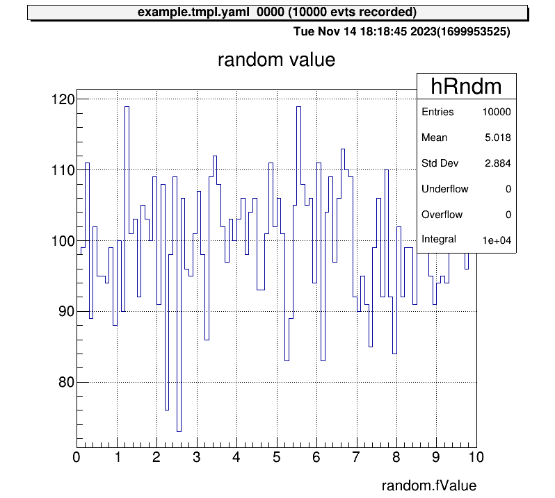
> 0 art::TH1FTreeProj hRndm random value
Here, art::TH1FTreeProj is a customized class derived from TH1F, designed for efficient analysis within artemis.
Drawing Histograms
Draw a histogram using the ht command with its ID or name:
artemis [] ht 0
To return to the root directory, use:
artemis [] cd
To move one directory up, use:
artemis [] cd ..
This moves you up one level in the directory structure.
Step 5: View Tree Data
After the event loop, a ROOT file containing tree objects is created.
List available files using fls:
artemis [] fls
 files
    0 TFile output/0001/example_0001.tree.root            (CREATE)
Navigate into the ROOT file using fcd with the file ID:
artemis [] fcd 0
Listing Branches
List tree branches with branchinfo (or br):
artemis [] br
random art::TSimpleData
View details of a branch’s members and methods:
artemis [] br random
art::TSimpleData

Data Members


Methods

                  Bool_t   CheckTObjectHashConsistency
            TSimpleData&   operator=
            TSimpleData&   operator=

See also

    art::TSimpleDataBase<double>
To explore inherited classes, use classinfo (or cl):
artemis [] cl art::TSimpleDataBase<double>
art::TSimpleDataBase<double>

Data Members

                  double   fValue

Methods

                    void   SetValue
                  double   GetValue
                  Bool_t   CheckTObjectHashConsistency
  TSimpleDataBase<double>&   operator=

See also

    art::TDataObject       base class for data object
Drawing Data from Trees
Unlike standard ROOT files, data in artemis cannot be accessed directly through branch names.
Instead, use member variables or methods of the branch objects.
Example:
artemis [] tree->Draw("random.fValue")
artemis [] tree->Draw("random.GetValue()")
VNC Server (option)
When performing data analysis, direct access to the server is not always practical. Many users connect via SSH, which can complicate graphical displays. While alternatives such as X11 forwarding or saving images exist, VNC is often preferred due to its lightweight design and fast rendering capabilities. This section explains how to set up and use a VNC server for visualization.
Setting Up the VNC Server
To use VNC, a VNC server must be installed on the analysis server.
Popular options include TigerVNC and TightVNC.
For CRIB analysis servers, TightVNC is the chosen implementation.
Installing TightVNC
To install TightVNC on an Ubuntu machine, use the following commands:
sudo apt update
sudo apt install tightvncserver
On CRIB servers, VNC is used solely to render artemis canvases. No desktop environment is installed. For further details, refer to the official TightVNC documentation.
Starting the VNC Server
Start the VNC server with the following command:
vncserver :10
Here, :10 specifies the display number, and the VNC server will run on port 5910 (calculated as 5900 + display number).
export DISPLAY=:10
However, sometimes you may find that even though VNC is running, the plot you’re trying to display does not appear. In this case, you should check the DISPLAY settings on the analysis computer.
Checking Active VNC Servers
If multiple VNC processes are active, using an already occupied display number will cause an error.
Check active VNC processes with the vnclist command, defined as an alias on CRIB servers:
vnclist
Example output:
Xtightvnc :23
Xtightvnc :3
Alias definition:
vnclist: aliased to pgrep -a vnc | awk '{print $2,$3}'
Configuring artemis to Use VNC
To render artemis canvases on the VNC server, the DISPLAY environment variable must be set correctly.
The a command automates this process.
How the a Command Works
The a command is defined as follows:
a() {
  if [ ! -e "artemislogon.C" ]; then
    printf "\033[1ma\033[0m: 'artemislogon.C' not found\n"
    return 1
  fi

  if [ -z "${SSH_CONNECTION:-}" ]; then
    artemis -l "$@"
  elif [ -f ".vncdisplay" ]; then
    DISPLAY=":$(cat .vncdisplay)" artemis -l "$@"
  else
    artemis -l "$@"
  fi
}
Explanation:
- If
artemislogon.Cis missing in the current directory, the command exits. - If not connected via SSH,
artemis -lruns using the local display. - If
.vncdisplayexists, its content is read to set theDISPLAYvariable before launchingartemis. - Otherwise,
artemis -lruns with default settings.
Configuring .vncdisplay
To direct artemis canvases to the VNC server:
- Create a
.vncdisplayfile in your working directory. - Add the display number (e.g.,
10) as its content:10 - Start
artemisusing theacommand. The canvas should now appear on the VNC server.
Configuring the VNC Client
To view canvases, you must connect to the VNC server using a VNC client. Popular options include RealVNC.
Connecting to the Server
If the client machine is on the same network as the server, connect using the server’s IP address (or hostname) and port number:
<analysis-server-ip>:5910
- The port number is
5900 + display number. - If prompted for a password, use the one set during the VNC server setup or contact the CRIB server administrator.
Using SSH Port Forwarding for Remote Access
When accessing the analysis server from an external network (e.g., from home), direct VNC connections are typically blocked. SSH port forwarding allows secure access in such cases.
flowchart LR;
    A("**Local Machine**")-->B("**SSH server**")
    B-->C("**Analysis Machine**")
    C-->B
    B-->A
Multi-Hop SSH Setup
If a gateway server is required for access, configure multi-hop SSH in your local machine’s .ssh/config file.
Example:
Host gateway
    HostName <gateway-server-ip>
    User <gateway-username>
    IdentityFile <path-to-private-key>
    ForwardAgent yes

Host analysis
    HostName <analysis-server-ip>
    User <analysis-username>
    IdentityFile <path-to-private-key>
    ForwardAgent yes
    ProxyCommand ssh -CW %h:%p gateway
    ServerAliveInterval 60
    ServerAliveCountMax 5
With this configuration, connect to the analysis server using:
ssh analysis
Setting Up Port Forwarding
To forward the analysis server’s VNC port (e.g., 5910) to a local port (e.g., 59010):
- Use the
-Loption in your SSH command:ssh -L 59010:<analysis-server-ip>:5910 analysis - Alternatively, add the
LocalForwardoption to your.ssh/configfile:Host analysis LocalForward 59010 localhost:5910 - After connecting via SSH, start your VNC client and connect to:
localhost:59010
You should now see the artemis canvases rendered on your local machine.
Note: This is one example configuration. Customize the setup as needed for your environment.
Steering Files
Steering files define the configuration for the data analysis flow in YAML format.
This section explains their structure and usage using the example file steering/example/example.tmpl.yaml from the previous section.
Understanding the Steering File
The content of steering/example/example.tmpl.yaml is structured as follows:
Anchor:
  - &treeout output/@NUM@/example_@NUM@.tree.root
  - &histout output/@NUM@/example_@NUM@.hist.root
Processor:
  - name: timer
    type: art::TTimerProcessor
  - include:
      name: rndm.inc.yaml
      replace:
        MAX: @MAX@
  - name: hist
    type: art::TTreeProjectionProcessor
    parameter:
      FileName: hist/example/example.hist.yaml
      OutputFilename: *histout
      Type: art::TTreeProjection
      Replace: |
        MAX: @MAX@
  - name: treeout
    type: art::TOutputTreeProcessor
    parameter:
      FileName: *treeout
The file is divided into two main sections:
Anchor: Defines reusable variables using the YAML anchor feature (&name value), which can be referenced later as*name.Processor: Specifies the sequence of processing steps for the analysis.
Variables Enclosed in @
Variables such as @NUM@ and @MAX@ are placeholders replaced dynamically when loading the steering file via the artemis command:
artemis [] add steering/example/example.tmpl.yaml NUM=0001 MAX=10
For example, the Anchor section is replaced as follows:
Anchor:
  - &treeout output/0001/example_0001.tree.root
  - &histout output/0001/example_0001.hist.root
This allows the steering file to adapt dynamically to different analysis configurations.
Data Processing Flow
When artemis runs, the processors defined in the Processor section are executed sequentially.
For example, the first processor in example.tmpl.yaml is:
- name: timer
  type: art::TTimerProcessor
Each processor entry requires the following keys:
name: A unique identifier for the process, aiding in debugging and logging.type: Specifies the processor class to use.parameter(optional): Defines additional parameters for the processor.
The general structure of any steering file is as follows:
- name: process1
  type: art::THoge1Processor
  parameter:
    prm1: hoge

- name: process2
  type: art::THoge2Processor
  parameter:
    prm2: hoge

- name: process3
  type: art::THoge3Processor
  parameter:
    prm3: hoge
Processors are executed in the order they appear in the file.
Referencing Other Steering Files
For modular or repetitive configurations, other steering files can be included using the include keyword.
For example:
  - include:
      name: rndm.inc.yaml
      replace:
        MAX: @MAX@
Content of rndm.inc.yaml
Processor:
  - name: MyTRandomNumberEventStore
    type: art::TRandomNumberEventStore
    parameter:
      Max: @MAX@  # [Float_t] the maximum value
      MaxLoop: 10000  # [Int_t] the maximum number of loops
      Min: 0  # [Float_t] the minimum value
      OutputCollection: random  # [TString] output name of random values
      OutputTransparency: 0  # [Bool_t] Output is persistent if false (default)
      Verbose: 1  # [Int_t] verbose level (default 1: non-quiet)
The flow of variable replacement is as follows:
MAX=10is passed via theartemiscommand.@MAX@inexample.tmpl.yamlis replaced with10.- The
replacedirective inexample.tmpl.yamlpropagates this value torndm.inc.yaml. @MAX@inrndm.inc.yamlis replaced with10.
Other Processing Steps
The remaining processors in the file handle histogram generation and saving data to a ROOT file:
  - name: hist
    type: art::TTreeProjectionProcessor
    parameter:
      FileName: hist/example/example.hist.yaml
      OutputFilename: *histout
      Type: art::TTreeProjection
      Replace: |
        MAX: @MAX@

  - name: treeout
    type: art::TOutputTreeProcessor
    parameter:
      FileName: *treeout
- Histogram generation is detailed in the next section.
- Output tree processing saves data to a ROOT file, utilizing aliases (
*treeout) defined in theAnchorsection.
General Structure of a Steering File
Steering files typically include the following processors:
- Timer: Measures processing time but does not affect data analysis.
- EventStore: Handles event information for loops.
- Mapping: Maps raw data to detectors.
- Processing steps: Performs specific data analysis tasks.
- Histogram: Generates histograms from processed data.
- Output: Saves processed data in ROOT file format.
flowchart LR
    A("**EventStore**") --> B("**Mapping**<br>(Optional)")
    B --> C("**Processing Steps**<br>(e.g., Calibration)")
    C --> D("**Histogram**<br>(Optional)")
    D --> E("**Output**")
    E -.-> |Loop| A
Summary
- Steering files define the analysis flow using YAML syntax.
- Dynamic variables enclosed in
@are replaced with command-line arguments. - The
Processorsection specifies the sequence of processing tasks. - Use
includeto reference other steering files for modular configurations. - Typical components include timers, data stores, mappings, processing steps, histograms, and output.
Histogram Definition
In the previous section, we introduced the structure of the steering file, including a processor for drawing histograms. In online analysis, quickly displaying predefined histograms is essential. This section explains how histograms are defined and managed.
Steering File Block
To process histograms, the art::TTreeProjectionProcessor is used (unless a custom processor has been created for CRIB).
Below is an example from steering/example/example.tmpl.yaml:
Processor:
  # skip
  - name: hist
    type: art::TTreeProjectionProcessor
    parameter:
      FileName: hist/example/example.hist.yaml
      OutputFilename: *histout
      Type: art::TTreeProjection
      Replace: |
        MAX: @MAX@
Key Parameters
- FileName: Points to the file with histogram definitions.
- OutputFilename: Specifies where the ROOT file containing the histogram objects will be saved. The YAML alias
*histoutis used here. - Type: Defines the processing class, which should be
art::TTreeProjectionfor histograms processed byart::TTreeProjectionProcessor. - Replace: Substitutes placeholders (e.g.,
@MAX@) in the histogram definition file with specified values.
Note: YAML's
|symbol ensures that line breaks are included as written. Though not critical in this case, it impacts multi-line text handling.
Histogram Definition File
The histogram definitions are stored in a separate file.
For instance, hist/example/example.hist.yaml contains:
group:
  - name: test
    title: test
    contents:
      - name: hRndm
        title: random value
        x: ["random.fValue",100,0.,@MAX@]

include:
  - name: hist/example/example.inc.yaml
    replace:
      MAX: @MAX@
      SUFFIX: 2
      BRANCH: random
The file is divided into two main blocks: group and include.
group Block
The group block organizes histograms into logical units.
Each group corresponds to an art::TTreeProjGroup object, which is referenced in the artemis command section:
artemis [] ls
 artemis
>   0 art::TTreeProjGroup test2           test (2)
    1 art::TTreeProjGroup test            test
    2 art::TAnalysisInfo analysisInfo
The name and title keys in the group block define the art::TTreeProjGroup object:
group:
  - name: test
    title: test
Defining Histogram Contents
Histograms within a group are defined under the contents key. Multiple histograms can be defined as an array. For example:
# skip
    contents:
      - name: hRndm
        title: random value
        x: ["random.fValue",100,0.,@MAX@]

      # you can add histograms here
      #- name: hRndm2
Key Parameters
| Key | Description |
|---|---|
| name | The histogram's unique identifier. |
| title | Display title for the histogram. |
| x | Defines the x-axis. Format: [variable, bin count, min, max]. |
| y | Defines the y-axis (if specified, creates a 2D histogram). |
| cut | Filter condition for the histogram, often referred to as a "cut" or "gate". |
variable in Histogram Definitions
Histograms generated by art::TTreeProjectionProcessor are created based on tree objects, similar to the ROOT command:
root [] tree->Draw("variable>>(100, -10.0, 10.0)", "variable2 > 1.0")
In this case:
- x:
["variable", 100, -10.0, 10.0] - cut:
"variable2 > 1.0;"
In artemis, data is accessed through the member variables or methods of branch objects rather than directly referencing branch names.
include Block
Histogram definition files can reference other files using the include keyword:
include:
  - name: hist/example/example.inc.yaml
    replace:
      MAX: @MAX@
      SUFFIX: 2
      BRANCH: random
- name: Specifies the path to the included file relative to the working directory.
- replace: Replaces placeholders in the included file with specified values.
Example of the referenced file hist/example/example.inc.yaml:
group:
  - name: test@SUFFIX@
    title: test (@SUFFIX@)
    contents:
      - name: hRndm@SUFFIX@
        title: random number
        x: ["@BRANCH@.fValue",100, 0., @MAX@]
The structure of the included file mirrors that of the main file. Conceptually, the included content is appended to the main file.
While the example code demonstrates referencing multiple files, overuse can lead to complexity. Reference files only when it simplifies management.
Summary
Histograms in artemis are defined through a combination of steering files and separate histogram definition files.
The art::TTreeProjectionProcessor processes these definitions, enabling efficient creation and display of histograms during analysis.
Key points:
- The steering file specifies the histogram processor and its parameters.
- Histogram definition files use
groupblocks to logically organize histograms and include key parameters likex,y, andcut. - External files can be included for reusability, but excessive inclusion should be avoided for clarity.
Preparation
Note: In CRIB analysis, processors introduced in this Chapter may be customized. they are discussed in the CRIB Chapter. Currently,
artemisitself was modified and rebuilt, but there is a possibility of developing equivalent processors within theart::cribnamespace in the future. If that occurs, this manual will need to be updated (okawak expected someone to do so).
Map and Seg Configuration
This section explains the necessary configurations for analyzing actual data. The structure of the data files assumes the RIDF (RIKEN Data File) format, commonly used in DAQ systems at RIKEN. Here, we focus on two essential configuration files for extracting and interpreting data: the map file and the segment file.
The Role of Configuration Files
In artemis, input data is stored in an object called the EventStore.
To process RIDF files, the class TRIDFEventStore is used.
Configuration files map the raw data in TRIDFEventStore to the corresponding DAQ modules and detectors, enabling accurate interpretation.
Segment Files
Segment files are used to read raw ADC or TDC data. When the map file is not properly configured, segment files help verify whether data exists in each channel.
Segment files are located in the conf/seg directory within your working directory.
The directory structure should look like this:
./
├── conf/
│   ├── map/
│   ├── seg/
│   │   ├── modulelist.yaml
│   │   ├── seglist.yaml
modulelist.yaml
The modulelist.yaml file defines the modules used in the analysis.
Each module corresponds to a DAQ hardware device, such as ADCs or TDCs.
Example: Configuration for a V1190A module
V1190A:
  id: 24
  ch: 128
  values:
    - tdcL: [300, -5000., 300000.] # Leading edge
    - tdcT: [300, -5000., 300000.] # Trailing edge
- V1190A: Module name, used in
seglist.yaml. - id: Module ID, defined in
TModuleDecoder(V1190 example) - ch: Total number of channels. For example, the V1190A module has 128 channels.
- values: Histogram parameters in the format
[bin_num, x_min, x_max]. These are used when checking raw data (see Raw data check).
seglist.yaml
The seglist.yaml file describes the settings of each module.
In the CRIB DAQ system (babirl), modules are identified using four IDs: dev, fp, mod, and geo.
These IDs are assigned during DAQ setup and are written into the RIDF data file.
ID Descriptions
| ID | Description | CRIB example |
|---|---|---|
| dev | Device ID: Distinguishes major groups (e.g., experiments). | CRIB modules use 12, BIGRIPS and SHARAQ use others. |
| fp | Focal Plane ID: Differentiates sections of the DAQ system or crates. | Common DAQ is used for CRIB focal planes, so this ID is used to differentiate MPV crates. |
| mod | Module ID: Identifies the purpose of the module (e.g., PPAC, PLA). | 6 for ADCs, 7 for TDCs, 63 for scalers. |
| geo | Geometry ID: Distinguishes individual modules with the same [dev, fp, mod] configuration. | Unique ID for each module. |
Example: Configuration for a V1190A module in seglist.yaml
J1_V1190:
  segid: [12, 2, 7]
  type: V1190A
  modules:
    - id: 0
    - id: 1
- J1_V1190: A descriptive name for the module, used when creating histograms or trees.
- segid: Represents [dev, fp, mod] values.
- type: Specifies the module type, as defined in
modulelist.yaml. - modules: Lists geometry IDs (geo). Multiple IDs can be specified as an array.
Map Files
Map files consist of a main configuration file (mapper.conf) and individual map files stored in the conf/map directory.
./
├── mapper.conf
├── conf/
│   ├── map/
│   │   ├── ppac/
│   │   │   ├── dlppac.map
│   │   ...
│   ├── seg/
mapper.conf
This file specifies which map files to load and their configuration. Each line in the file indicates the path to a map file relative to the working directory and the number of columns of the segid in the file. Example configuration:
# file path for configuration, relative to the working directory
# (path to the map file) (Number of columns)

#====================================
# bld
# cid = 1: rf
conf/map/rf/rf.map 1

# cid = 2: coin
conf/map/coin/coin.map 1

# cid = 3: f1ppac
conf/map/ppac/f1ppac.map 5

# cid = 4: dlppac
conf/map/ppac/dlppac.map 5
Format of the mapper.conf
- Path: Specifies the relative path to the map file.
- Number of Columns: Indicates the number of segments defined in the map file.
Individual Map Files
Each map file maps DAQ data segments to detector inputs. The general format is:
cid, id, [dev, fp, mod, geo, ch], [dev, fp, mod, geo, ch], ...
ID description
| ID | Description |
|---|---|
catid or cid | Category ID: Groups data for specific analysis. |
detid or id | Detector ID: Differentiates datasets within a category. It corresponds to the row of map files. |
[dev, fp, mod, geo, ch] | Represents segment IDs and channels (segid). |
typeid | Index of the segment IDs. The first set of segid is correspond to 0. |
Example for dlppac.map:
# map for dlppac
#
#  Map: X1 X2 Y1 Y2 A
#
#--------------------------------------------------------------------
# F3PPACb
   4,   0,  12,   2,  7,   0,   4,  12,   2,  7,   0,   5,  12,   2,  7,   0,   6,  12,   2,  7,   0,   7,  12,   2,  7,   0,   9
# F3PPACa
   4,   1,  12,   0,  7,   16,   1,  12,   0,  7,   16,   2,  12,   0,  7,   16,   3,  12,   0,  7,   16,   4,  12,   0,  7,   16,   0
In this example:
catid = 4: Indicates the PPAC category.detid = 0, 1: Identifies the specific data set within this category.- Five
[dev, fp, mod, geo, ch]combinations: Define the five input channels (X1, X2, Y1, Y2, A). typeid = 0corresponds X1,typeid = 1corresponds X2, and so on.
Relation to mapper.conf
The number of [dev, fp, mod, geo, ch] combinations in a map file determines the column count in mapper.conf.
For example:
conf/map/ppac/dlppac.map 5
Verifying the Mapping (Optional)
To ensure correctness, use the Python script pyscripts/map_checker.py:
python pyscripts/map_checker.py
For uv environments:
uv run pyscripts/map_checker.py
Summary
- Segment files: Define hardware modules and verify raw data inputs (refer to Raw Data Check).
- Map files: Map DAQ data to detectors and analysis inputs. Verify with
map_checker.py.
Read RIDF Files
This section explains how to read RIDF files using artemis.
Currently, binary RIDF files are processed using two classes: art::TRIDFEventStore and art::TMappingProcessor.
Using art::TRIDFEventStore to Read Data
To load data from a RIDF file, use art::TRIDFEventStore.
Here is an example of a steering file:
Anchor:
  - &input ridf/@NAME@@NUM@.ridf
  - &output output/@NAME@/@NUM@/hoge@NAME@@NUM@.root
  - &histout output/@NAME@/@NUM@/hoge@NAME@@NUM@.hist.root

Processor:
  - name: timer
    type: art::TTimerProcessor

  - name: ridf
    type: art::TRIDFEventStore
    parameter:
      OutputTransparency: 1
      Verbose: 1
      MaxEventNum: 100000
      SHMID: 0
      InputFiles:
        - *input

  - name: outputtree
    type: art::TOutputTreeProcessor
    parameter:
      FileName:
        - *output
The timer processor shows analysis time and is commonly included.
The key section to note is the ridf block.
Key Parameters
| Parameter | Defalut Value | Description |
|---|---|---|
| OutputTransparency | 0 | 0 saves output to a ROOT file, 1 keeps it for internal use only. (Inherited from art::TProcessor.) |
| Verbose | 1 | 0 for quiet mode, 1 for detailed logs. (Inherited from art::TProcessor.) |
| MaxEventNum | 0 | 0 for no limit; otherwise specifies the number of entries to process. |
| SHMID | 0 | Shared Memory ID for DAQ in online mode (babirl nssta mode). |
| InputFiles | Empty array | List of input RIDF file paths. Files are processed sequentially into a single ROOT file. |
Unspecified parameters use default values.
Parameters inherited from art::TProcessor are common to all processors.
Processing with art::TRIDFEventStore
The objects processed by this processor are difficult to handle directly.
It is common to set OutputTransparency to 1, meaning the objects will not be saved to a ROOT file.
To understand what is produced, you can set OutputTransparency to 0 to examine the output.
artlogin <username>
a
artemis [] add steering/hoge.yaml NAME=xxxx NUM=xxxx
artemis [] res
artemis [] sus
artemis [] fcd 0
artemis [] br
For detailed commands, refer to the Artemis Commands section.
Example output:
segdata              art::TSegmentedData
eventheader          art::TEventHeader
The eventheader is always output, while segdata is produced when OutputTransparency is set to 0.
Key data is contained in segdata.
Further details are covered in subsequent sections.
Using art::TMappingProcessor for Data Mapping
Raw RIDF files do not inherently indicate detector associations or processing rules. Use mapping files, as explained in the previous section, to map the data.
Example steering file:
Processor:
  - name: timer
    type: art::TTimerProcessor

  - name: ridf
    type: art::TRIDFEventStore
    parameter:
      OutputTransparency: 1
      Verbose: 1
      MaxEventNum: 100000
      SHMID: 0
      InputFiles:
        - *input

  - name: mapper
    type: art::TMappingProcessor
    parameter:
      OutputTransparency: 1
      MapConfig: mapper.conf

  - name: outputtree
    type: art::TOutputTreeProcessor
    parameter:
      FileName:
        - *output
Key Parameters
| Parameter | Defalut Value | Description |
|---|---|---|
| MapConfig | mapper.conf | Path to the mapper configuration file. Defaults to mapper.conf in the working directory. |
This parameter allows custom mappings, such as focusing on specific data during standard analyses.
Use an alternative mapper.conf in another directory and specify its path when needed.
Processing with art::TMappingProcessor
The outputs of this processor are also hard to use directly, so OutputTransparency is typically set to 1.
To examine what is produced, set it to 0 and observe the output.
artlogin <username>
a
artemis [] add steering/hoge.yaml NAME=xxxx NUM=xxxx
artemis [] res
artemis [] sus
artemis [] fcd 0
artemis [] br
Example output:
segdata              art::TSegmentedData
eventheader          art::TEventHeader
catdata              art::TCategorizedData
A new branch, catdata, is created.
It categorizes data from segdata and serves as the basis for detector-specific analyses.
Workflow Diagram
flowchart LR
    A("**RIDF data files**") --> B("<u>**art::TRIDFEventStore**</u><br>input: RIDF files<br>output: segdata")
    B --> C("<u>**art::TMappingProcessor**</u><br>input: segdata<br>output: catdata")
    C --> D("**<u>Mapping Processor</u>**<br>input: catdata<br>output: hoge")
    D --> E("**<u>Other Processors</u>**<br>input: hoge<br>output: fuga")
    C --> F("**<u>Mapping Processor</u>**<br>input: catdata<br>output: foo")
    F --> G("**<u>Other Processors</u>**<br>input: foo<br>output: bar")
Both segdata and catdata are typically set to OutputTransparency: 1 and processed internally.
Understanding these objects is essential for mastering subsequent analyses.
Time Reference for V1190
At CRIB, the CAEN V1190 module is used to acquire timing data in Trigger Matching Mode, where timing data within a specified window is recorded upon receiving a trigger signal.
The raw data from the module includes module-specific uncertainties. To ensure accurate timing, corrections are required. This section explains how to apply these corrections.
Raw Data
To understand the behavior of the V1190, consider the following setup:
flowchart LR
    subgraph V1190
        direction TB
        B("**Module**")
        C("Channels")
    end
    A("**Trigger Making**")-->|trigger|B
    A-->|data|C
    A-->|tref|C
- The trigger signal is input directly to the V1190, and timing data is recorded using two channels.
- The recorded data is referred to as
dataandtref.
When data is examined without corrections, the result looks like this:
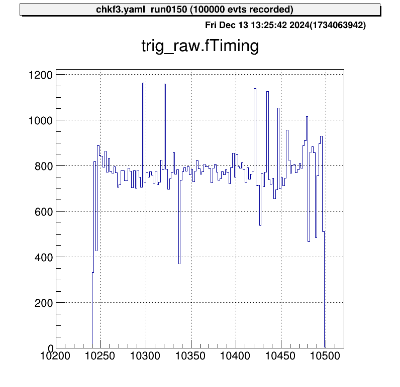
The horizontal axis represents the V1190 channel numbers. In this example, one channel corresponds to approximately 0.1 ns, leading to an uncertainty of about 25 ns. Ideally, since this signal is a trigger, data points should align at nearly the same channel.
Correction Using "Tref"
This uncertainty is consistent across all data recorded by the V1190 for the same event, meaning it is fully correlated across channels.
By subtracting a reference timing value (called tref) from all channels, this module-specific uncertainty can be corrected.
Below is an example of corrected data after subtracting tref:
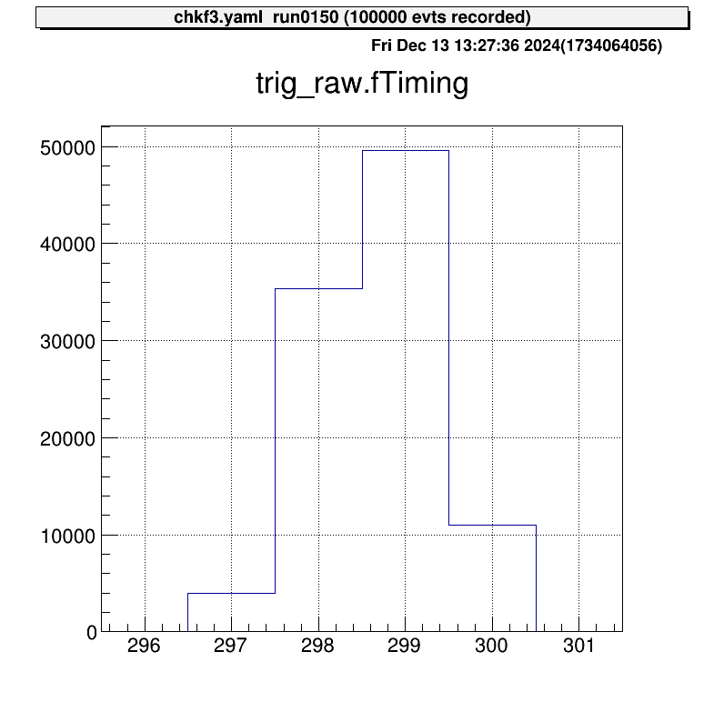
The trigger signal now aligns at nearly the same channel. Without this correction, V1190-specific uncertainties degrade resolution, making this correction essential.
Any signal can be used as a
tref, but it must be recorded some signals for all events. For simplicity, the trigger signal is often used astref.
Applying the Correction in Steering Files
The correction is implemented using the steering/tref.yaml file, which is maintained separately for easy reuse.
An example configuration is shown below:
Processor:
  # J1 V1190A
  - name: proc_tref_v1190A_j1
    type: art::TTimeReferenceProcessor
    parameter:
      # [[device] [focus] [detector] [geo] [ch]]
      RefConfig: [12, 2, 7, 0, 0]
      SegConfig: [12, 2, 7, 0]
Tref Processor Workflow
- Use the
art::TTimeReferenceProcessor. - Specify
RefConfig(tref channel) andSegConfig(target module). - The processor subtracts the channel specified in
RefConfigfrom all data in the module identified bySegConfig.
Refer to the ID scheme to correctly configure RefConfig and SegConfig for your DAQ setup.
Adding the Tref Processor to the Main Steering File
Include the tref processor in the main steering file using the include keyword.
Ensure the tref correction is applied before processing other signals. For example:
Anchor:
  - &input ridf/@NAME@@NUM@.ridf
  - &output output/@NAME@/@NUM@/hoge@NAME@@NUM@.root
  - &histout output/@NAME@/@NUM@/hoge@NAME@@NUM@.hist.root

Processor:
  - name: timer
    type: art::TTimerProcessor

  - name: ridf
    type: art::TRIDFEventStore
    parameter:
      OutputTransparency: 1
      InputFiles:
        - *input
      SHMID: 0

  - name: mapper
    type: art::TMappingProcessor
    parameter:
      OutputTransparency: 1

  # Apply tref correction before other signal processing
  - include: tref.yaml

  # Process PPAC data with corrected timing
  - include: ppac/dlppac.yaml

  - name: outputtree
    type: art::TOutputTreeProcessor
    parameter:
      FileName:
        - *output
PPAC Calibration
MWDC Calibration
The current author (okawak) is not familiar with the MWDC, so please wait for further information from someone else.
Alpha-Source Calibration
MUX Calibration
Starting with the 2025 version, the structure of MUX parameter files and their loading method have been updated. Please note that these changes are not backward-compatible with earlier versions.
At CRIB, we use the MUX module by Mesytec. This multiplexer circuit is designed for strip-type Si detectors and consolidates five outputs:
- Two energy outputs (
E1,E2), - Two position outputs (
P1,P2) for identifying the corresponding strip, - One timing output (
T) from the discriminator.
The MUX can handle up to two simultaneous hits per trigger, outputting them as E1, E2, and P1, P2.
In single-hit events, E2 and P2 remain empty.
Currently, handling for E2 and P2 outputs is not implemented.
In practice, most Si detector events involve a single hit per trigger, and coincidence events have not posed a problem.
If you need to process E2 and P2, additional handling must be implemented.
This guide explains how to process data using the MUX in detail.
Map File
Since the five outputs are processed as a single set, the segid in the map file is written in five columns.
Update the mapper.conf as follows:
conf/map/ssd/tel_dEX.map 5
In the map file, list the segid values in the order [E1, E2, P1, P2, T]:
# Map: MUX [ene1, ene2, pos1, pos2, timing]
#
#--------------------------------------------------------------------
40,  0, 12  1  6   4   16, 12  1  6   4   17, 12  1  6   4   18, 12  1  6   4   19, 12  2  7  0   70
In this example, you can access these data sets using catid 40.
Checking Raw Data
To inspect raw data, use the art::crib::TMUXDataMappingProcessor:
Processor:
  - name: MyTMUXDataMappingProcessor
    type: art::crib::TMUXDataMappingProcessor
    parameter:
      CatID: -1 # [Int_t] Category ID
      OutputCollection: mux # [TString] Name of the output branch
Key Parameters
CatID: Thecatidspecified in the map file.OutputCollection: The name of the output branch.
Accessing TMUXData Type
| Name | Variable | Getter |
|---|---|---|
| E1 | fE1 | GetE1() |
| E2 | fE2 | GetE2() |
| P1 | fP1 | GetP1() |
| P2 | fP2 | GetP2() |
| T | fTiming (first hit) | GetTrig() |
| T | fTVec[idx] (timing array) | GetT(idx) |
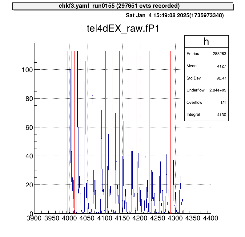
For example, to examine the P1 position signal:
artlogin <username>
a
artemis [] add steering/hoge.yaml NAME=xxxx NUM=xxxx
artemis [] res
artemis [] sus
artemis [] fcd 0
artemis [] zo
artemis [] tree->Draw("mux.fP1")
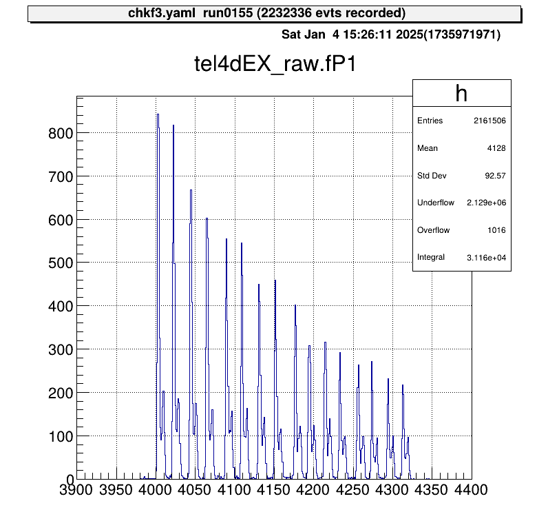
The position output appears as discrete signals, with each peak corresponding to a strip number.
If the map file includes multiple rows:
40,  0, 12  1  6   4   16, 12  1  6   4   17, 12  1  6   4   18, 12  1  6   4   19, 12  2  7  0   70
40,  1, 12  1  6   4   20, 12  1  6   4   21, 12  1  6   4   22, 12  1  6   4   23, 12  2  7  0   71
The output will be a two-element array.
To process this further, use art::TSeparateOutputProcessor to split the array into individual elements.
The YAML array index corresponds to the row in the map file:
Processor:
  - name: MyTSeparateOutputProcessor
    type: art::TSeparateOutputProcessor
    parameter:
      InputCollection: inputname # [TString] name of input collection
      OutputCollections: # [StringVec_t] list of name of output collection
        - mux1
        - mux2
Calibration
What Is MUX Calibration?
To calibrate a detector using a MUX circuit, the position output must be mapped to its corresponding strip, and each event assigned to the correct strip.
In the current method, as illustrated, an event falling into two adjacent regions (from the left) is assigned to the corresponding x-th strip.
The goal of MUX calibration is to determine the red boundary values in the figure and save them in a parameter file.
Calibration Macros
To streamline the MUX calibration process, two macros are provided:
macro/run_MUXParamMaker.C: Runs the calibration macro and logs its execution.macro/MUXParamMaker.C: Contains the core function for performing MUX calibration.
The main calibration function, defined in macro/MUXParamMaker.C, requires the following arguments:
h1: Histogram object.telname: Telescope name for specifying the output directory.sidename: Indicates whether it’s the X or Y direction strip ("dEX"or"dEY"), also used for directory naming.runname、runnum: Used to generate the output file name to distinguish between different measurements.peaknum: Number of expected peaks (currently assumes 16 strips).
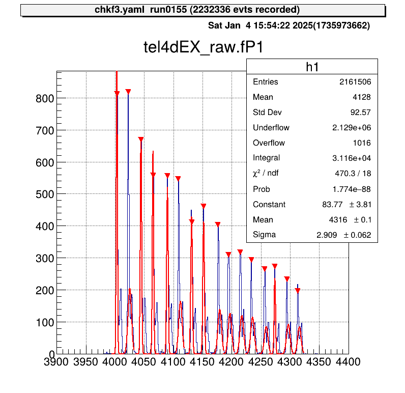
In macro/run_MUXParamMaker.C, use the ProcessLine() function to define calibration commands:
void run_MUXParamMaker() {
    const TString ARTEMIS_WORKDIR = gSystem->pwd();

    const TString RUNNAME = "run";
    const TString RUNNUM = "0155";

    gROOT->ProcessLine("fcd 0");
    gROOT->ProcessLine("zone");

    gROOT->ProcessLine("tree->Draw(\"tel4dEX_raw.fP1>>h1(500,3900.,4400.)\")");
    gROOT->ProcessLine(".x " + ARTEMIS_WORKDIR + "/macro/MUXParamMaker.C(h1, \"tel4\", \"dEX\", \"" + RUNNAME + "\", \"" + RUNNUM + "\", 16)");
}
This macro records the calibration conditions.
To use it:
artemis [] add steering/hoge.yaml NAME=xxxx NUM=xxxx
artemis [] res
artemis [] sus
artemis [] .x macro/run_MUXParamMaker.C
Gaussian fitting is performed on each peak, and the parameter file is saved automatically.
Applying Parameters
Parameter files are stored in directories like prm/tel[1,2,...]/pos_dE[X, Y]/.
To simplify access, predefined steering files use a symbolic link called current.
By changing this symbolic link, you can switch parameter files without modifying the steering file.
Use the setmuxprm.sh script to manage these symbolic links.
This script requires gum and realpath.
Run the script interactively to create a current link pointing to the desired parameter file:
./setmuxprm.sh
Verifying Parameters
To verify the parameters, use the macro/chkmuxpos.C macro.
- Generate a histogram of
P1in Artemis. - Overlay the boundary lines from the current parameter file.
artlogin <username>
a
artemis [] add steering/hoge.yaml NAME=xxxx NUM=xxxx
artemis [] res
artemis [] sus
artemis [] fcd 0
artemis [] tree->Draw("mux.fP1>>h1")
To draw the boundaries on the histogram h1:
artemis [] .x macro/chkmuxpos.C(h1, "telname", "sidename")
Arguments:
h1: Histogram object.telname: Telescope name, used for locating the parameter file.sidename: Specify"dEX"or"dEY", also used for locating the parameter file.
This visual representation helps confirm that each peak aligns with its designated region.
Energy Calibration
Energy calibration is performed on a strip-by-strip basis, so strip assignment must be completed beforehand.
Parameter Objects
To load the necessary parameters into Artemis and use them in a processor, employ the art::TParameterArrayLoader:
Processor:
  - name: proc_@NAME@_dEX_position
    type: art::TParameterArrayLoader
    parameter:
      Name: prm_@NAME@_dEX_position
      Type: art::crib::TMUXPositionConverter
      FileName: prm/@NAME@/pos_dEX/current
      OutputTransparency: 1
Processor Parameters:
Name: Specifies the name of the parameter object.Type: Specifies the class type of the parameter.FileName: Path to the parameter file.OutputTransparency: Set to 1 since parameter objects do not need to be saved in ROOT files.
Strip Assignment with TMUXCalibrationProcessor
Strip assignment is handled using the art::crib::TMUXCalibrationProcessor:
Processor:
  - name: MyTMUXDataMappingProcessor
    type: art::crib::TMUXDataMappingProcessor
    parameter:
      CatID: -1 # [Int_t] Category ID
      OutputCollection: mux_raw # [TString] Name of the output branch

  - name: MyTMUXCalibrationProcessor
    type: art::crib::TMUXCalibrationProcessor
    parameter:
      InputCollection: mux_raw # [TString] Array of TMUXData objects
      OutputCollection: mux_cal # [TString] Output array of TTimingChargeData objects
      ChargeConverterArray: no_conversion # [TString] Energy parameter object of TAffineConverter
      TimingConverterArray: no_conversion # [TString] Timing parameter object of TAffineConverter
      PositionConverterArray: prm_@NAME@_dEX_position # [TString] Position parameter object of TMUXPositionConverter
      HasReflection: 0 # [Bool_t] Reverse strip order (0--7) if true
Note: In CRIB, the Y-direction strip numbering for silicon detectors differs between geometric and output pin order. Set
HasReflectiontoTrueto reverse the strip order and align it with the natural geometric sequence.
The PositionConverterArray parameter is mandatory for strip assignment.
Energy and timing converters are optional; if left unspecified, the raw values are returned.
Performing Energy Calibration
The objects output by art::crib::TMUXCalibrationProcessor (mux_cal) are of type art::TTimingChargeData.
The fID field corresponds to the detid (i.e., the strip number).
Therefore, energy calibration can be conducted in a manner similar to the Alpha Calibration section.
Important: Perform energy calibration using the output from the calibration processor, not the mapping processor.
Summary
- MUX Calibration: Aligns the position output with the corresponding strips by determining and storing boundary values in parameter files.
- Parameter Loading: Use
art::TParameterArrayLoaderto load parameters for strip assignment into Artemis. - Strip Assignment: Employ
art::crib::TMUXCalibrationProcessorto complete strip assignment before performing energy calibration. - Calibration Workflow:
PositionConverterArrayis required for strip assignment.- Energy and timing converters are optional; raw values are used if not specified.
- Energy Calibration: Conducted on the processor output to ensure proper alignment of detector strips.
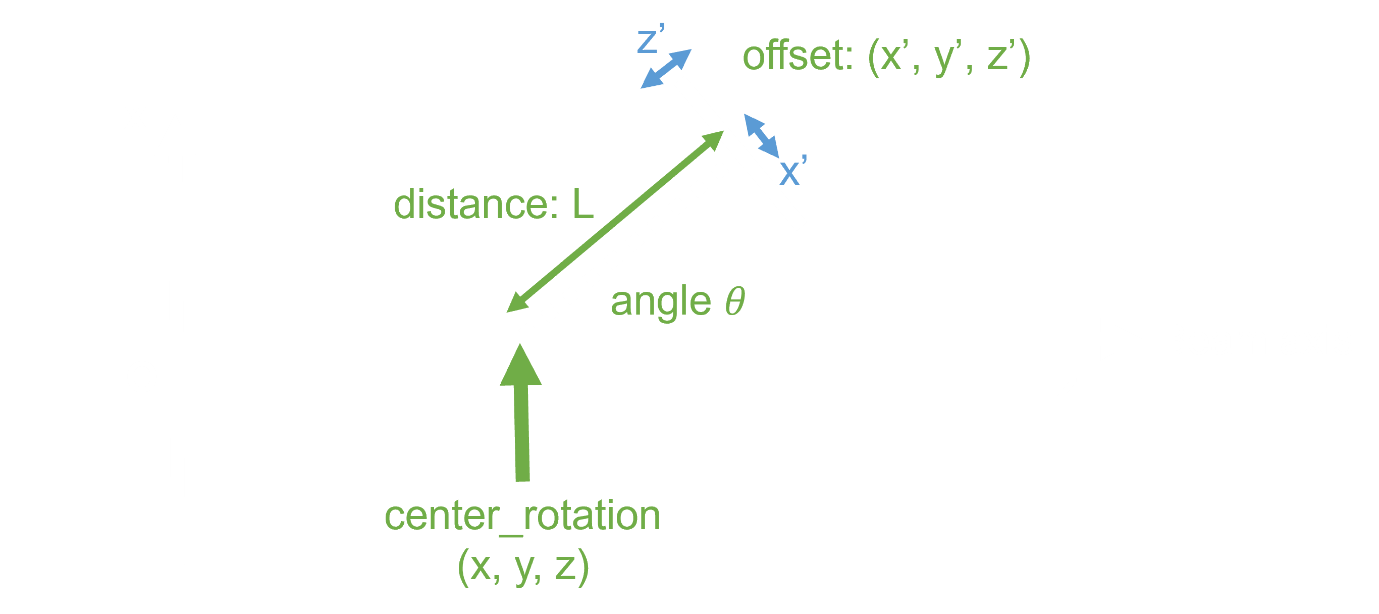
Geometry Setting
Git Operations (option)
CRIB Own Configuration
Analysis Environments
Online-mode Analysis
User Config
New Commands
Minor Change
Online Analysis
F1 Analysis
F2 Analysis
PPAC Analysis
MWDC Analysis
The current author (okawak) is not familiar with the MWDC, so please wait for further information from someone else.
Telescopes Analysis
F3 Analysis
Raw Data Check
Gate Processor
Shifter Tasks
Scaler Monitor
TimeStamp Treatment
Creating New Processors
The source code in artemis is categorized into several types.
The names below are unofficial and were introduced by okawak:
- Main: The primary file for creating the executable binary for artemis.
- Loop: Manages the event loop.
- Hist: Handles histograms.
- Command: Defines commands available in the artemis console.
- Decoder: Manages decoders and their configurations.
- EventStore: Handles events used in the event loop.
- EventCollection: Manages data and parameter objects.
- Processor: Processes data.
- Data: Defines data structures.
- Parameter: Manages parameter objects.
- Others: Miscellaneous files, such as those for artemis canvas or other utilities for analysis.
While users are free to customize these components, this chapter focuses on the Processor and Data categories, as these are often essential for specific analyses.
This chapter provides a step-by-step demonstration of creating a new processor and explains art::TRIDFEventStore and art::TMappingProcessor in detail, a crucial component for building processors.
Contents
-
A brief introduction to
EventStore. This section does not cover how to create or use a newEventStore. -
An overview of key concepts shared by all processors.
-
Explains
segdataproduced byart::TRIDFEventStoreand demonstrates how to use it to build a new processor. -
Describes Mapping Processors, which map data based on
catdataoutput fromart::TMappingProcessor. This section also provides a detailed explanation ofcatdata. -
Explains how to define new data classes. In artemis, specific classes are typically stored as elements in ROOT's
TClonesArray. This section details how to define data structures for this purpose. -
Explains how to define parameters for data analysis, either as member variables within a processor or as standalone objects usable across multiple processors.
EventStore
For previous CRIB analyses, the following three types of EventStore provided by artemis have been sufficient:
art::TRIDFEventStore: Reads RIDF files.art::TTreeEventStore: Reads ROOT files.art::TRandomNumberEventStore: Outputs random numbers.
If you need to create a new EventStore, these files can serve as useful examples.
General Processors
To process data in artemis, you need to define a class that inherits from art::TProcessor and implement specific data processing logic.
Since artemis integrates with ROOT, the class must also be registered in the ROOT dictionary, requiring some adjustments beyond standard C++ conventions.
This section explains the common settings and methods that should be implemented when creating any processor.
Header File
We will use an example of a simple processor named art::crib::THogeProcessor.
The prefix T follows ROOT naming conventions.
The header file is named THogeProcessor.h as this extension is conventionally used in artemis.
1. Include Guard
Use an include guard to prevent multiple inclusions of the header file.
Although #pragma once is an alternative, a token-based include guard is recommended for broader compatibility.
#ifndef _CRIB_THOGEPROCESSOR_H_
#define _CRIB_THOGEPROCESSOR_H_

#endif
2. Include TProcessor.h
Include the base class art::TProcessor to inherit its functionality.
Forward declarations are not sufficient for inheritance.
#include <TProcessor.h>
3. Forward Declarations
Use forward declarations for classes defined elsewhere to minimize dependencies. This approach reduces compilation overhead.
class TClonesArray;

namespace art {
class TSegmentedData;
class TCategorizedData;
} // namespace art
4. Class Definition
Classes developed for CRIB should use the art::crib namespace and inherit from art::TProcessor.
Although inline namespace declarations like class art::crib::THogeProcessor are possible, using a namespace block improves readability.
namespace art::crib {
class THogeProcessor : public TProcessor {
};
} // namespace art::crib
Note: The inline namespace syntax (
art::crib) is standardized in C++17.
5. Class Methods
Define essential methods for a processor, such as constructors, destructors, and overridden methods from art::TProcessor.
class THogeProcessor : public TProcessor {
  public:
    THogeProcessor();
    ~THogeProcessor();

    void Init(TEventCollection *col) override;
    void Process() override;
    void EndOfRun() override;
};
- Override additional virtual methods based on your analysis requirements.
Refer to the
art::TProcessorimplementation for a full list of available methods. - Use the
overridekeyword to ensure clarity and correctness.
6. Copy Constructor and Assignment Operator
Disable copy constructors and assignment operators as they are not used in artemis.
class THogeProcessor : public TProcessor {
  private:
    THogeProcessor(const THogeProcessor &) = delete;
    THogeProcessor &operator=(const THogeProcessor &) = delete;
};
7. Member Variables
Define member variables as private or protected unless they need external access.
Use pointers for forward-declared classes.
class THogeProcessor : public TProcessor {
  private:
    TClonesArray **fInData;
    TSegmentedData **fSegmentedData;
    TCategorizedData **fCategorizedData;

    Int_t fCounter;
    Int_t fIntParameter;
};
8. ROOT-Specific Features
To integrate the class with ROOT, follow these conventions:
- Add
//!(or///<!for Doxygen comment) to pointer-to-pointer members to exclude them from ROOT's streaming mechanism (TStreamer). - Use
ClassDefOverrideif the class hasoverridemethods; otherwise, useClassDef.
The macro’s second argument indicates the class version. Increment the version number when making changes to maintain compatibility.
class THogeProcessor : public TProcessor {
  private:
    TClonesArray **fInData;              //!
    TSegmentedData **fSegmentedData;     //!
    TCategorizedData **fCategorizedData; //!

    Int_t fCounter;
    Int_t fIntParameter;

    ClassDefOverride(THogeProcessor, 0);
};
Note: Adding
;after ROOT macros, though not required, improves readability.
Complete Header File Example
#ifndef _CRIB_THOGEPROCESSOR_H_
#define _CRIB_THOGEPROCESSOR_H_

#include "TProcessor.h"

class TClonesArray;

namespace art {
class TSegmentedData;
class TCategorizedData;
} // namespace art

namespace art::crib {
class THogeProcessor : public TProcessor {
  public:
    THogeProcessor();
    ~THogeProcessor();

    void Init(TEventCollection *col) override;
    void Process() override;
    void EndOfRun() override;

  private:
    TClonesArray **fInData;              //!
    TSegmentedData **fSegmentedData;     //!
    TCategorizedData **fCategorizedData; //!

    Int_t fCounter;
    Int_t fIntParameter;

    THogeProcessor(const THogeProcessor &) = delete;
    THogeProcessor &operator=(const THogeProcessor &) = delete;

    ClassDefOverride(THogeProcessor, 0);
};
} // namespace art::crib

#endif // end of #ifndef _CRIB_THOGEPROCESSOR_H_
Source File
Save the implementation in a file named THogeProcessor.cc.
1. Include the Header File
Include the header file with double quotes.
#include "THogeProcessor.h"
2. ClassImp Macro
Use the ClassImp macro to register the class with ROOT.
Add ; for consistency.
ClassImp(art::crib::THogeProcessor);
3. Use a Namespace Block
Wrap implementations within the art::crib namespace.
namespace art::crib {
// Implementation goes here
}
4. Implement Class Methods
Constructor
The constructor is called when an instance of the class is created.
It initializes member variables and registers parameters using methods like RegisterProcessorParameter().
THogeProcessor::THogeProcessor() : fInData(nullptr), fSegmentedData(nullptr), fCategorizedData(nullptr), fCounter(0) {
    RegisterProcessorParameter("IntParameter", "an example parameter read from steering file",
                               fIntParameter, 0);
}
RegisterProcessorParameter() links a parameter in the steering file to a member variable.
It accepts four arguments:
- Parameter Name: The name used in the steering file.
- Description: A brief description of the parameter.
- Variable Reference: The variable to assign the parameter value.
- Default Value: The default value used if the parameter is not specified in the steering file.
This method is implemented using templates, allowing it to accept variables of different types. Other functions for registering parameters will be explained later as needed, on a case-by-case basis.
Destructor
The destructor is called when the instance is destroyed. Release resources if needed in the destructor.
THogeProcessor::~THogeProcessor() {
}
Init() Method
Called before the event loop begins, when you command add steering/hoge.yaml.
void THogeProcessor::Init(TEventCollection *) {
    Info("Init", "Parameter: %d", fIntParameter);
}
- Use ROOT’s logging functions, such as
Info(),Warning(), andError(), inherited fromTObject.
Process() Method
Handles event-by-event processing.
void THogeProcessor::Process() {
    fCounter++;
    Info("Process", "Event Number: %d", fCounter);
}
EndOfRun() Method
Finalizes processing after the event loop ends.
void THogeProcessor::EndOfRun() {
}
Complete Source File Example
#include "THogeProcessor.h"

ClassImp(art::crib::THogeProcessor);

namespace art::crib {
THogeProcessor::THogeProcessor() : fInData(nullptr), fSegmentedData(nullptr), fCategorizedData(nullptr), fCounter(0) {
    RegisterProcessorParameter("IntParameter", "an example parameter read from steering file",
                               fIntParameter, 0);
}

THogeProcessor::~THogeProcessor() {
}

void THogeProcessor::Init(TEventCollection *) {
    Info("Init", "Parameter: %d", fIntParameter);
}

void THogeProcessor::Process() {
    fCounter++;
    Info("Process", "Event Number: %d", fCounter);
}

void THogeProcessor::EndOfRun() {
}

} // namespace art::crib
Registering the Class
Add the new class to the src-crib/artcrib_linkdef.h file for dictionary registration:
// skip
#pragma link C++ class art::crib::THogeProcessor;
// skip
Various processors are already registered, so you can copy the line and replace it with the name of your own class.
Build Configuration
Update src-crib/CMakeLists.txt to include the new files:
set(CRIBSOURCES
    # skip
    THogeProcessor.cc
    # skip
   )

set(CRIBHEADERS
    # skip
    THogeProcessor.h
    # skip
    )
Rebuild the project:
artlogin <username>
cd build
cmake ..
make -j4
make install
Additional Comments
Existing processors may have less optimal implementations as they were created when the author (okawak) was less experienced with C++. Feel free to improve them.
If you create a new processor or modify an existing one for future CRIB use, document its usage here or include Doxygen comments in the code. Clear documentation is vital for future team members to maintain and use the tool effectively.
Processing Segmented Data
This section explains how to create a processor, TChannelSelector, to extract specific channel data from segdata and store it in a TTree.
Along the way, we will explore the structure and contents of segdata.
For more details on how segdata is generated, see Read RIDF files.
Processor Overview
flowchart LR
    A("**RIDF data files**") --> B("<u>**art::TRIDFEventStore**</u><br>input: RIDF files<br>output: segdata")
    B --> C{"<u>**art::crib::TChannelSelector**</u>"}
We aim to create a processor with the following specifications:
- Name:
TChannelSelector - Namespace:
art::crib(specific to CRIB development) - Input:
segdata - Output: A branch, containing a
TClonesArrayofart::TSimpleDataobjects.
Note: The current implementation of art::TOutputTreeProcessor does not support writing primitive data types (e.g.,
intordouble) to branches. Instead, we useart::TSimpleData(a class with a single memberfValue) and wrap it in aTClonesArray.
Example Steering File
Below is an example structure for the steering file:
Anchor:
  - &input ridf/@NAME@@NUM@.ridf
  - &output output/@NAME@/@NUM@/test@NAME@@NUM@.root

Processor:
  - name: timer
    type: art::TTimerProcessor

  - name: ridf
    type: art::TRIDFEventStore
    parameter:
      OutputTransparency: 1
      InputFiles:
        - *input

  - name: channel
    type: art::crib::TChannelSelector
    parameter:
      parameter: hoge # add later

  - name: outputtree
    type: art::TOutputTreeProcessor
    parameter:
      FileName:
        - *output
Initial Setup
-
Create header and source files for
TChannelSelectorfollowing General Processors. Ensure that the class is registered inartcrib_linkdef.handCMakeLists.txt. -
Build and install the project to confirm the skeleton files work correctly:
artlogin <username>
cd build
cmake ..
make
make install
- Verify that artemis starts without errors:
acd
a
# -> No errors
Understanding segdata
Accessing segdata
To access segdata, add the following member variables to the header file:
class TChannelSelector : public TProcessor {
  private:
    TString fSegmentedDataName; // Name of the input object
    TSegmentedData **fSegmentedData; //! Pointer to the segdata object

    ClassDefOverride(TChannelSelector, 0);
};
Next, register the input collection name in the constructor using RegisterInputCollection:
TChannelSelector::TChannelSelector() : fSegmentedData(nullptr) {
    RegisterInputCollection("SegmentedDataName", "name of the segmented data",
                            fSegmentedDataName, TString("segdata"));
}
Explanation of Arguments:
- Name: Used in the steering file to specify the parameter.
- Description: A brief explanation of the variable.
- Variable: Stores the parameter's value
- Default value: Used if the parameter is not set in steering file.
Finally, retrieve the actual object in the Init method:
#include <TSegmentedData.h>

void TChannelSelector::Init(TEventCollection *col) {
    void** seg_ref = col->GetObjectRef(fSegmentedDataName);
    if (!seg_ref) {
        SetStateError(Form("No such input collection '%s'\n", fSegmentedDataName.Data()));
        return;
    }

    auto *seg_obj = static_cast<TObject *>(*seg_ref);
    if (!seg_obj->InheritsFrom("art::TSegmentedData")) {
        SetStateError(Form("'%s' is not of type art::TSegmentedData\n", fSegmentedDataName.Data()));
        return;
    }

    fSegmentedData = reinterpret_cast<TSegmentedData **>(seg_obj);
}
Step-by-Step Explanation:
-
Retrieve Object Reference: Use
GetObjectRef(returnvoid **) to retrieve the object associated with the name infSegmentedDataName. If the object is not found, log an error and exits. -
Validate Object Type: Check that the object inherits from
art::TSegmentedDatausingInheritsFrom. This ensures compatibility during casting. -
Store Object: Cast the object to
TSegmentedDataand store it infSegmentedDatafor later use.
Exploring segdata Structure
art::TSegmentedData inherits from TObjArray, with each entry corresponding to a [dev, fp, mod] tuple.
The following code outputs the structure of segdata for each event:
void TChannelSelector::Process() {
    auto nSeg = fSegmentedData->GetEntriesFast();
    for (int iSeg = 0; iSeg < nSeg; iSeg++) {
        auto *seg = fSegmentedData->UncheckedAt(iSeg);

        int id = seg->GetUniqueID();
        // id is generated by `id = (dev << 20) + (fp << 14) + (mod << 8)`
        int dev = (id >> 20) & 0xFFF;
        int fp = (id >> 14) & 0x3F;
        int mod = (id >> 8) & 0x3F;

        std::cout << "iSeg=" << iSeg << ", [dev=" << dev << ", fp=" << fp << ", mod=" << mod << "]\n";
    }
}
Example output:
iSeg=0, [dev=12, fp=1, mod=6]
iSeg=1, [dev=12, fp=1, mod=60]
iSeg=2, [dev=12, fp=2, mod=7]
...
Decoded Data Overview
The following table summarizes the decoded data classes used for different modules:
| Module | Class | Description |
|---|---|---|
| V7XX (V775, V785) | art::TRawTiming | Inherits from art::TRawDataObject -> art::TRawDataSimple -> art::TRawTiming. Although the name indicates timing data, ADC data are also handled by this class. |
| MXDC32 (MADC32) | art::TRawTiming | Same as above. |
| V1190 | art::TRawTimingWithEdge | Inherits from art::TRawTiming -> art::TRawTimingWithEdge. This class is designed to handle both leading edge and trailing edge timing data. |
These modules are commonly used in CRIB experiments. Note that other type the modules such as scaler are not covered in this page.
Key Features:
- Unified Access: All decoded objects inherit from
art::TRawDataObject, allowing consistent access methods. - Virtual Functions: Access data (e.g.,
geo,ch,val) using the same methods across different modules.
Extracting Specific Segments
To extract data for a specific segment ([dev, fp, mod]), use FindSegment:
#include <TRawDataObject.h>

void TChannelSelector::Process() {
    auto *seg_array = fSegmentedData->FindSegment(12, 0, 7);
    if (!seg_array) {
        Warning("Process", "No segment having segid = [dev=12, fp=0, mod=7]");
        return;
    }

    auto nData = seg_array->GetEntriesFast();
    for (int iData = 0; iData < nData; iData++) {
        auto *data = (TRawDataObject *)seg_array->UncheckedAt(iData);
        int geo = data->GetGeo();
        int ch = data->GetCh();
        int val = data->GetValue();
        std::cout << "iData=" << iData << ", [geo=" << geo << ", ch=" << ch << ", val=" << val << "]\n";
    }
}
Process Explanation
- Retrieve Segment Array:
The
FindSegmentmethod (returnTObjArray *) contains all entries for the specified segment ID ([dev, fp, mod]). If the segment does not exist, a warning is logged, and the method exits. - Iterate Through Entries:
Each entry in the segment array represents a data point for the specified segment.
Use
UncheckedAtorAtto access individual entries and extract properties likegeo,ch, andvalusing methods ofart::TRawDataObject.
Example output:
iData=0, [geo=0, ch=2, val=9082]
iData=1, [geo=0, ch=2, val=9554]
iData=2, [geo=0, ch=0, val=25330]
iData=3, [geo=0, ch=0, val=26274]
iData=4, [geo=1, ch=2, val=9210]
iData=5, [geo=1, ch=2, val=9674]
iData=6, [geo=1, ch=0, val=25449]
...
Implementing TChannelSelector
Preparing Parameters
To specify the target segment and channels, add a SegID parameter ([dev, fp, mod, geo, ch]) in the steering file:
- name: channel
  type: art::crib::TChannelSelector
  parameter:
    SegID: [12, 0, 7, 0, 2]
Implementation:
-
Declare Member Variable: Add a member variable to the header file to store the
SegIDparameter:class TChannelSelector : public TProcessor { private: IntVec_t fSegID; //! } -
Register Parameter: Use
RegisterProcessorParameterin the constructor to read the parameter from the steering file:TChannelSelector::TChannelSelector() : fSegmentedData(nullptr) { IntVec_t init_i_vec; RegisterProcessorParameter("SegID", "segment ID, [dev, fp, mod, geo, ch]", fSegID, init_i_vec); } -
Validate Parameter: Validate the
SegIDsize in theInitmethod:void TChannelSelector::Init(TEventCollection *col) { if (fSegID.size() != 5) { SetStateError("parameter: SegID size is not 5, input [dev, fp, mod, geo, ch]\n"); return; } Info("Init", "Process [dev=%d, fp=%d, mod=%d, geo=%d, ch=%d]", fSegID[0], fSegID[1], fSegID[2], fSegID[3], fSegID[4]); }
Preparing Output Branch
To store extracted data, create a ROOT branch using TClonesArray:
-
Declare Member Variables: Add member variables for the output branch in the header file:
class TChannelSelector : public TProcessor { private: TString fOutputColName; TClonesArray *fOutData; //! } -
Register Output Collection: Register the branch name in the constructor:
TChannelSelector::TChannelSelector() : fSegmentedData(nullptr), fOutData(nullptr) { RegisterOutputCollection("OutputCollection", "name of the output branch", fOutputColName, TString("output")); } -
Steering File: Add
SegIDparameter in the steering file:- name: channel type: art::crib::TChannelSelector parameter: OutputCollection: channel SegID: [12, 0, 6, 0, 2] # add this parameter -
Initialize Output Branch: Initialize the
TClonesArrayobject in theInitmethod:#include <TSimpleData.h> void TChannelSelector::Init(TEventCollection *col) { fOutData = new TClonesArray("art::TSimpleData"); fOutData->SetName(fOutputColName); col->Add(fOutputColName, fOutData, fOutputIsTransparent); Info("Init", "%s -> %s", fSegmentedDataName.Data(), fOutputColName.Data()); }
Processing Events
Process events to extract and store data matching the specified SegID:
-
Clear Data: Ensure the output branch is cleared for each event:
void TChannelSelector::Process() { fOutData->Clear("C"); } -
Extract and Store Data: Use the following logic to extract and store data in
TClonesArray:
void TChannelSelector::Process() {
    auto *seg_array = fSegmentedData->FindSegment(fSegID[0], fSegID[1], fSegID[2]);
    if (!seg_array) {
        Warning("Process", "No segment having segid = [dev=%d, fp=%d, mod=%d]", fSegID[0], fSegID[1], fSegID[2]);
        return;
    }

    auto nData = seg_array->GetEntriesFast();
    int counter = 0;
    for (int iData = 0; iData < nData; ++iData) {
        auto *data = (TRawDataObject *)seg_array->UncheckedAt(iData);
        int geo = data->GetGeo();
        int ch = data->GetCh();
        if (data && geo == fSegID[3] && ch == fSegID[4]) {
            auto *outData = static_cast<art::TSimpleData *>(fOutData->ConstructedAt(counter));
            counter++;
            outData->SetValue(data->GetValue());
        }
    }
}
Explanation:
- Clear Output:
fOutData->Clear("C")ensures no residual data from the previous event. - Filter Data: Only entries matching
geoand ch values fromSegIDare processed. - Store Data: Use
ConstructedAt(counter)to create new entries in the TClonesArray.
Verifying the Implementation
After completing the implementation, use the following commands to test the processor:
artemis [] add steering/hoge.yaml NAME=xxxx NUM=xxxx
artemis [] res
artemis [] sus
artemis [] fcd 0
artemis [] tree->Scan("channel.fValue")
Example Output:
***********************************
*    Row   * Instance * channel.f *
***********************************
*        0 *        0 *      9314 *
*        0 *        1 *      9818 *
*        1 *        0 *           *
*        2 *        0 *      3842 *
*        2 *        1 *      4550 *
*        3 *        0 *           *
*        4 *        0 *      8518 *
*        4 *        1 *      9107 *
*        5 *        0 *           *
*        6 *        0 *           *
See the complete implementation:
Processing Categorized Data
This section explains how to create a new processor using categorized data (catdata) generated by art::TMappingProcessor.
Such processors are referred to as Mapping Processors.
The classification of data is defined in the mapper.conf and conf/map files.
For details on creating map files, see Map Configuration.
In this section, we will:
- Create a processor to extract specific data defined in the map file and store it in
art::TSimpleData. - Explore the structure of
catdata.
The overall process is similar to what was discussed in the previous section.
Processor Overview
flowchart LR
    A("**RIDF data files**") --> B("<u>**art::TRIDFEventStore**</u><br>input: RIDF files<br>output: segdata")
    B --> C("<u>**art::TMappingProcessor**</u><br>input: segdata<br>output: catdata")
    C --> D{"<u>**art::crib::TMapSelector**</u>"}
We will create the following processor:
- Name:
TMapSelector - Namespace:
art::crib(for CRIB-specific code) - Input:
catdata - Output: A branch with elements of
art::TSimpleDatastored in aTClonesArray
Map File Example
A sample map file looks like this:
10, 0,  12 1  6   3  0,  12 2  7  0  16
10, 1,  12 1  6   3  1,  12 2  7  0  17
In this format:
- The first column specifies the
catid. - The second column specifies the
detid. - Subsequent groups of five numbers represent
segidvalues, withtypeiddifferentiating between these groups.
For example, specifying CatID: [10, 1, 1] extracts segid = [12, 2, 7, 0, 17].
Example Steering File
A steering file is used to define parameters like CatID and the output branch name.
Below is a sample configuration:
Anchor:
  - &input ridf/@NAME@@NUM@.ridf
  - &output output/@NAME@/@NUM@/test@NAME@@NUM@.root

Processor:
  - name: timer
    type: art::TTimerProcessor

  - name: ridf
    type: art::TRIDFEventStore
    parameter:
      OutputTransparency: 1
      InputFiles:
        - *input

  - name: mapper
    type: art::TMappingProcessor
    parameter:
      OutputTransparency: 1

  - name: map_channel
    type: art::crib::TMapSelector
    parameter:
      OutputCollection: channel
      CatIDs: [10, 1, 1]

  - name: outputtree
    type: art::TOutputTreeProcessor
    parameter:
      FileName:
        - *output
Working with catdata
Creating TMapSelector
Begin by creating the header and source files for TMapSelector.
Don’t forget to register these files in artcrib_linkdef.h and CMakeLists.txt.
For details, refer to the General processor.
Header File
The header file defines the required components and variables for handling catdata:
#ifndef _CRIB_TMAPSELECTOR_H_
#define _CRIB_TMAPSELECTOR_H_

#include "TProcessor.h"

class TClonesArray;

namespace art {
class TCategorizedData;
} // namespace art

namespace art::crib {
class TMapSelector : public TProcessor {
  public:
    TMapSelector();
    ~TMapSelector();

    void Init(TEventCollection *col) override;
    void Process() override;

  private:
    TString fCategorizedDataName;
    TString fOutputColName;

    IntVec_t fCatID; //! [cid, id, type]

    TCategorizedData **fCategorizedData; //!
    TClonesArray *fOutData;             //!

    TMapSelector(const TMapSelector &) = delete;
    TMapSelector &operator=(const TMapSelector &) = delete;

    ClassDefOverride(TMapSelector, 1);
};
} // namespace art::crib

#endif // end of #ifndef _CRIB_TMAPSELECTOR_H_
Source File
Prepare the source file to receive catdata in a manner similar to how segdata is handled.
The Process() method will be implemented later.
#include "TMapSelector.h"

#include <TCategorizedData.h>
#include <TRawDataObject.h>
#include <TSimpleData.h>

ClassImp(art::crib::TMapSelector);

namespace art::crib {
TMapSelector::TMapSelector() : fCategorizedData(nullptr), fOutData(nullptr) {
    RegisterInputCollection("CategorizedDataName", "name of the segmented data",
                            fCategorizedDataName, TString("catdata"));
    RegisterOutputCollection("OutputCollection", "name of the output branch",
                             fOutputColName, TString("channel"));

    IntVec_t init_i_vec;
    RegisterProcessorParameter("CatID", "Categorized ID, [cid, id, type]",
                               fCatID, init_i_vec);
}

void TMapSelector::Init(TEventCollection *col) {
    // Categorized data initialization
    void** cat_ref = col->GetObjectRef(fCategorizedDataName);
    if (!cat_ref) {
        SetStateError(Form("No input collection '%s'", fCategorizedDataName.Data()));
        return;
    }

    auto *cat_obj = static_cast<TObject *>(*cat_ref);
    if (!cat_obj->InheritsFrom("art::TCategorizedData")) {
        SetStateError(Form("Invalid input collection '%s': not TCategorizedData",
                           fCategorizedDataName.Data()));
        return;
    }
    fCategorizedData = reinterpret_cast<TCategorizedData **>(cat_ref);

    // CatID validation
    if (fCatID.size() != 3) {
        SetStateError("CatID must contain exactly 3 elements: [cid, id, type]");
        return;
    }

    fOutData = new TClonesArray("art::TSimpleData");
    fOutData->SetName(fOutputColName);
    col->Add(fOutputColName, fOutData, fOutputIsTransparent);
    Info("Init", "%s -> %s, CatID = %d",
         fCategorizedDataName.Data(), fOutputColName.Data(), fCatID[0]);
}
} // namespace art::crib
Structure of catdata
catdata is a hierarchical object composed of nested TObjArray instances. For further details, refer to the TCategorizedData.cc implementation.
The structure can be visualized as follows:
catdata (Array of categories)
├── [Category 0] (TObjArray)
│    ├── [Detector 0] (TObjArray)
│    │    ├── [Type 0] (TObjArray)
│    │    │    ├── TRawDataObject
│    │    │    ├── TRawDataObject
│    │    │    └── ...
│    │    ├── [Type 1] (TObjArray)
│    │    │    ├── TRawDataObject
│    │    │    └── ...
│    │    └── ...
│    └── [Detector 1] (TObjArray)
│         ├── [Type 0] (TObjArray)
│         └── ...
├── [Category 1] (TObjArray)
│    └── ...
└── ...
Key relationships:
- Category corresponds to the first column (
catid) in the map file. - Detector ID corresponds to the second column (
detid). - Type identifies the specific group (
segid) referred to.
Extracting a Category (catid)
To retrieve a specific category, use the FindCategory(catid) method:
TObjArray* det_array = categorizedData->FindCategory(catid);
This returns an array corresponding to a row in the map file.
Extracting a Detector ID (detid, id)
To retrieve a specific detid from the category array, access it using:
TObjArray* type_array = (TObjArray*) det_array->At(index);
Note: The index does not directly correspond to the detid.
The actual detid value is stored within the object and must be accessed programmatically.
Extracting Data (from type)
To extract data (art::TRawDataObject) from the type_array, use the following:
TObjArray* data_array = (TObjArray*) type_array->At(typeIndex);
TRawDataObject* data = (TRawDataObject*) data_array->At(dataIndex);
The type_array is created using the AddAtAndExpand method of TObjArray, meaning its size corresponds to the map file and can be accessed by index.
Each element in type_array is also a TObjArray, designed to handle multi-hit TDC data.
Use the At method to access individual elements and cast them to TRawDataObject.
Displaying Data
Here is an example of how to extract and display data for a specific catid, such as catid = 7:
void TMapSelector::Process() {
    if (!fCategorizedData) {
        Warning("Process", "No CategorizedData object");
        return;
    }

    auto *cat_array = fCategorizedData->FindCategory(7); // Specify catid
    if (!cat_array)
        return;

    const int nDet = cat_array->GetEntriesFast();
    for (int iDet = 0; iDet < nDet; ++iDet) {
        auto *det_array = static_cast<TObjArray *>(cat_array->At(iDet));
        const int nType = det_array->GetEntriesFast();
        for (int iType = 0; iType < nType; ++iType) {
            auto *data_array = static_cast<TObjArray *>(det_array->At(iType));
            const int nData = data_array->GetEntriesFast();
            for (int iData = 0; iData < nData; ++iData) {
                auto *data = dynamic_cast<TRawDataObject *>(data_array->At(iData));
                int id = data->GetSegID();
                // id is generated by `id = (dev << 20) + (fp << 14) + (mod << 8)`
                int dev = (id >> 20) & 0xFFF;
                int fp = (id >> 14) & 0x3F;
                int mod = (id >> 8) & 0x3F;

                std::cout << "dev=" << dev << " fp=" << fp << " mod=" << mod << " geo=" << data->GetGeo() << " ch=" << data->GetCh()
                          << " : catid=" << data->GetCatID() << " detid=" << data->GetDetID() << " typeid=" << data->GetType()
                          << " : detIndex=" << iDet << " typeIndex=" << iType << " dataIndex=" << iData << std::endl;
            }
        }
    }
}
Example Output:
dev=12 fp=0 mod=7 geo=1 ch=75 : catid=7 detid=25 typeid=0 : detIndex=0 typeIndex=0 dataIndex=0
dev=12 fp=0 mod=7 geo=1 ch=75 : catid=7 detid=25 typeid=0 : detIndex=0 typeIndex=0 dataIndex=1
dev=12 fp=0 mod=7 geo=1 ch=84 : catid=7 detid=54 typeid=0 : detIndex=1 typeIndex=0 dataIndex=0
dev=12 fp=0 mod=7 geo=1 ch=84 : catid=7 detid=54 typeid=0 : detIndex=1 typeIndex=0 dataIndex=1
dev=12 fp=0 mod=7 geo=1 ch=84 : catid=7 detid=54 typeid=0 : detIndex=1 typeIndex=0 dataIndex=2
dev=12 fp=0 mod=7 geo=1 ch=84 : catid=7 detid=54 typeid=0 : detIndex=1 typeIndex=0 dataIndex=3
...
Implementing TMapSelector
The Process() method extracts data for a specific channel, matching detid (fCatID[1]) and storing values in art::TSimpleData.
Error handling is omitted for brevity.
void TMapSelector::Process() {
    fOutData->Clear("C");

    auto *cat_array = fCategorizedData->FindCategory(fCatID[0]);
    const int nDet = cat_array->GetEntriesFast();
    int counter = 0;
    for (int iDet = 0; iDet < nDet; ++iDet) {
        auto *det_array = static_cast<TObjArray *>(cat_array->At(iDet));
        auto *data_array = static_cast<TObjArray *>(det_array->At(fCatID[2]));
        const int nData = data_array->GetEntriesFast();
        for (int iData = 0; iData < nData; ++iData) {
            auto *data = dynamic_cast<TRawDataObject *>(data_array->At(iData));
            if (data && data->GetDetID() == fCatID[1]) {
                auto *outData = static_cast<art::TSimpleData *>(fOutData->ConstructedAt(counter));
                counter++;
                outData->SetValue(data->GetValue());
            }
        }
    }
}
Verification
To verify consistency with the previous section (TChannelSelector), compare the extracted catid and segid using the following commands:
artlogin <usename>
a
artemis [] add steering/hoge.yaml NAME=xxxx NUM=xxxx
artemis [] res
artemis [] sus
artemis [] fcd 0
artemis [] tree->Scan("channel.fValue:mapchannel.fValue")
Example Output:
***********************************************
*    Row   * Instance * channel.f * mapchanne *
***********************************************
*        0 *        0 *     20843 *     20843 *
*        0 *        1 *     21394 *     21394 *
*        1 *        0 *           *           *
*        2 *        0 *           *           *
*        3 *        0 *     19049 *     19049 *
*        3 *        1 *     19665 *     19665 *
*        4 *        0 *           *           *
*        5 *        0 *           *           *
*        6 *        0 *     24904 *     24904 *
*        6 *        1 *     25490 *     25490 *
*        7 *        0 *           *           *
For full implementation details, see:
Data Classes
In previous examples, we used art::TSimpleData, which stores a single fValue element, as an item in a TClonesArray.
When handling more complex data structures, you need to define custom data classes.
This page explains how to design a data class using art::crib::TMUXData as an example.
Finally, we demonstrate how to use TMUXData in a mapping processor to pack data from catdata into the TMUXData structure for MUX data.
Designing TMUXData
Step 1: Include Guards
Add a unique include guard to the header file to prevent multiple inclusions.
#ifndef _CRIB_TMUXDATA_H
#define _CRIB_TMUXDATA_H

#endif // _CRIB_TMUXDATA_H
Step 2: Namespace Block
Define the class within the art::crib namespace to ensure proper organization.
namespace art::crib {
} // namespace art::crib
Step 3: Class Definition
All Artemis data classes must inherit from art::TDataObject.
Include this header file and define the basic class structure:
#include <TDataObject.h>

namespace art::crib {
class TMUXData : public TDataObject {
  public:
    TMUXData();
    ~TMUXData();
    TMUXData(const TMUXData &rhs);
    TMUXData &operator=(const TMUXData &rhs);

    void Copy(TObject &dest) const override;
    void Clear(Option_t *opt = "") override;
  private:
    ClassDefOverride(TMUXData, 1);
};
} // namespace art::crib
This class includes:
- Constructor and destructor
- Copy constructor and assignment operator
CopyandClearmethods (required for all data classes)
The ClassDef macro enables ROOT to manage the class.
Step 4: Data Structure Design
MUX modules output five types of data as a group: [E1, E2, P1, P2, T].
Define a structure to store these values in one object.
class TMUXData : public TDataObject {
  public:
    // Getter and Setter
    Double_t GetE1() const { return fE1; }
    void SetE1(Double_t value) { fE1 = value; }
    Double_t GetE2() const { return fE2; }
    void SetE2(Double_t value) { fE2 = value; }
    Double_t GetP1() const { return fP1; }
    void SetP1(Double_t value) { fP1 = value; }
    Double_t GetP2() const { return fP2; }
    void SetP2(Double_t value) { fP2 = value; }
    Double_t GetTrig() const { return fTiming; }
    void SetTrig(Double_t value) { fTiming = value; }

    static const Int_t kNRAW = 5;

  private:
    Double_t fE1;
    Double_t fE2;
    Double_t fP1;
    Double_t fP2;
    Double_t fTiming;
};
Store the data in private member variables and provide access through getters and setters.
Step 5: Implement Methods
Implement the required methods in the source file. These include:
- Initializing member variables in the constructor
- Implementing the destructor (if necessary)
- Copy constructor and assignment operator
CopyandClearmethods
Additionally, handle the logic of the parent class art::TDataObject.
#include "TMUXData.h"

#include <constant.h> // for kInvalidD and kInvalidI

ClassImp(art::crib::TMUXData);

namespace art::crib {
TMUXData::TMUXData()
    : fE1(kInvalidD), fE2(kInvalidD),
      fP1(kInvalidD), fP2(kInvalidD),
      fTiming(kInvalidD) {
    TDataObject::SetID(kInvalidI);
}

TMUXData::~TMUXData() = default;

TMUXData::TMUXData(const TMUXData &rhs)
    : TDataObject(rhs),
      fE1(rhs.fE1),
      fE2(rhs.fE2),
      fP1(rhs.fP1),
      fP2(rhs.fP2),
      fTiming(rhs.fTiming) {
}

TMUXData &TMUXData::operator=(const TMUXData &rhs) {
    if (this != &rhs) {
        TDataObject::operator=(rhs);
        fE1 = rhs.fE1;
        fE2 = rhs.fE2;
        fP1 = rhs.fP1;
        fP2 = rhs.fP2;
        fTiming = rhs.fTiming;
    }
    return *this;
}

void TMUXData::Copy(TObject &dest) const {
    TDataObject::Copy(dest);
    auto *cobj = dynamic_cast<TMUXData *>(&dest);
    cobj->fE1 = this->GetE1();
    cobj->fE2 = this->GetE2();
    cobj->fP1 = this->GetP1();
    cobj->fP2 = this->GetP2();
    cobj->fTiming = this->GetTrig();
}

void TMUXData::Clear(Option_t *opt) {
    TDataObject::Clear(opt);
    TDataObject::SetID(kInvalidI);
    fE1 = kInvalidD;
    fE2 = kInvalidD;
    fP1 = kInvalidD;
    fP2 = kInvalidD;
    fTiming = kInvalidD;
}
} // namespace art::crib
These methods ensure that the data class is properly initialized, copied, and cleared during its lifecycle.
Designing TMUXDataMappingProcessor
With the TMUXData class created, we can now use it in an actual processor.
This section also explains the general structure of the Process() function in a Mapping Processor.
For detailed information, refer to Mapping Processors.
Selecting the Category ID
The Category ID (catid) groups detectors or data requiring similar processing.
Unlike the TMapSelector processor introduced earlier, all data within a single catid is generally processed together in a single processor.
// fCatID: Int_t
const auto *cat_array = fCategorizedData->FindCategory(fCatID);
All data in this cat_array will be used within the processor.
Iterating Through Detector IDs
To access all data within cat_array, iterate using a for loop:
const int nDet = cat_array->GetEntriesFast();
    for (int iDet = 0; iDet < nDet; ++iDet) {
        const auto *det_array = static_cast<const TObjArray *>(cat_array->At(iDet));
    }
Note: The
detidspecified in the map file does not directly match the array index.
You can retrieve the detid from art::TRawDataObject and store it in the art::crib::TMUXData object:
// data : art::crib::TMUXData*
int detID = data->GetDetID();
muxData->SetID(detID);
SetID is defined in the parent class art::TDataObject.
When interacting with the object in Artemis, use fID for access:
detid<->fID
Example:
artemis [] tree->Draw("obj.fID")
Accessing TRawDataObject
To retrieve a data object from det_array:
const auto *data_array = static_cast<const TObjArray *>(det_array->At(iType));
const auto *data = dynamic_cast<const TRawDataObject *>(data_array->At(0));
For multi-hit TDCs, where multiple data points exist in a single segment, the size of data_array increases.
When receiving data from catdata (as a Mapping Processor), the data is handled as art::TRawDataObject.
Storing Data in the Output Object
To store data in the output object defined in Init() or similar functions, allocate memory using TClonesArray's ConstructedAt(idx):
auto *outData = static_cast<TMUXData *>(fOutData->ConstructedAt(idx));
outData->SetE1(raw_data[0]);
outData->SetE2(raw_data[1]);
outData->SetP1(raw_data[2]);
outData->SetP2(raw_data[3]);
outData->SetTrig(raw_data[4]);
Here, the output object is cast to art::crib::TMUXData, and the data is stored using the defined setters.
For the next event, clear the values by calling:
fOutData->Clear("C");
This invokes the Clear() function defined in art::crib::TMUXData.
Ensure that all elements are correctly cleared; otherwise, data from previous events might persist.
Proper implementation of the Clear() function is essential.
Summary
- TMUXData: A custom data class tailored for MUX data.
- TMUXDataMappingProcessor: Demonstrates how to process and store data using the custom class.
- Group data by
catidand access it usingdetid. - Process raw data (
TRawDataObject) and store it inTMUXData.
- Group data by
- Key Considerations:
- Use
SetIDto storedetidand access it consistently withfID. - Implement the
Clear()function correctly to avoid processing errors in subsequent events.
- Use
This guide completes the design and usage of TMUXData and its integration into a mapping processor.
The example provides a solid foundation for handling more complex data structures in similar workflows.
Parameter Objects (Converters)
A Parameter Object is an object that stores strings or numeric values loaded from a parameter file. This section focuses on Converters, which use these parameters to transform one value into another, such as for calibration purposes.
In the Artemis framework, these objects are managed using the art::TParameterArrayLoader processor.
While the art::TParameterLoader processor handles non-array parameters, art::TParameterArrayLoader can process single-element arrays, making it more versatile.
The art::TParameterArrayLoader packs a specific parameter type into a TClonesArray, enabling other processors to access it.
To use this feature, you need to define a custom parameter object type to be stored in the TClonesArray.
For instance, to transform a value value using the first element of the parameter object in the TClonesArray:
auto converted_value = (prm->At(0))->Convert(value);
Here, the Convert method performs the transformation.
This guide demonstrates how to implement a Converter, focusing on the art::crib::TMUXPositionConverter, which converts MUX position output to strip numbers.
We’ll also explore its application in the art::crib::TMUXCalibrationProcessor.
Understanding TParameterArrayLoader
Before creating a custom parameter class, it's important to understand how art::TParameterArrayLoader works.
Processor:
  - name: MyTParameterArrayLoader
    type: art::TParameterArrayLoader
    parameter:
      FileFormat: text # [TString] file format : text (default), yaml
      FileName: path/to/file # [TString] input filename
      Name: parameter # [TString] name of parameter array output
      OutputTransparency: 0 # [Bool_t] Output is persistent if false (default)
      Type: art::TParameterObject # [TString] type(class) of parameter
      Verbose: 1 # [Int_t] verbose level (default 1 : non quiet)
While the FileFormat can be set to yaml for YAML files, this guide focuses on reading numeric values from text files.
For details on YAML processing, refer to the art::TParameterArrayLoader implementation.
The class specified in the Type field of the steering file will be implemented in later sections.
Reading from a Text File
The FileName field in the steering file specifies the text file to read.
The following is the relevant snippet from the loader’s implementation (error handling excluded):
Bool_t TParameterArrayLoader::LoadText() {
   std::ifstream fin(fFileName.Data());
   TParameterObject *parameter = nullptr;
   TString buf;
   Int_t count = 0;
   while(buf.ReadLine(fin)) {
      if (!parameter) {
         parameter =
            static_cast<TParameterObject*>(fParameterArray->ConstructedAt(count));
      }

      if (parameter->LoadString(buf)) {
         parameter = nullptr;
         ++count;
      }
   }
   fin.close();
   if(!count)
      return kFALSE;
   fParameterArray->Expand(count);
   return kTRUE;
}
Key Points
buf.ReadLine(fin): Reads the file line by line.- For each line, a new parameter object element is created using
ConstructedAt.
- For each line, a new parameter object element is created using
LoadString(): Processes a single line of text.- If
LoadString()returnstrue, thecountvariable increments, preparing for the next object. - This is a virtual method in
art::TParameterObjectthat must be overridden in custom classes.
- If
Defining a Custom Parameter Class
All parameter objects must inherit from art::TParameterObject.
To use the Convert method, extend art::TConverterBase, which declares the virtual Convert() method.
#include <TConverterBase.h>

namespace art::crib {
class TMUXPositionConverter : public TConverterBase {
  public:
    TMUXPositionConverter();
    ~TMUXPositionConverter();

    Double_t Convert(Double_t val) const override;
    Bool_t LoadString(const TString &str) override;
    void Print(Option_t *opt = "") const override;

  private:
    std::vector<Double_t> fParams;

    ClassDefOverride(TMUXPositionConverter, 0);
};
} // namespace art::crib
This class overrides the following methods:
Convert: Performs value transformation.LoadString: Reads and processes a single line from the text file.
Implementation in Source File
In the source file, provide specific implementations for the Convert and LoadString methods.
These methods handle the transformation logic and file parsing, respectively.
namespace art::crib {
Double_t TMUXPositionConverter::Convert(const Double_t val) const {
    // Define the specific transformation logic
}

Bool_t TMUXPositionConverter::LoadString(const TString &str) {
    // Define the specific transformation logic
}
} // namespace art::crib
Note: Design the structure of the parameter file before implementation to ensure compatibility. Reviewing examples in the following sections can help you visualize how the Converter will be used.
Using Parameter Classes
This section demonstrates how to use parameter classes to create a processor that performs value transformations.
First, use art::TParameterArrayLoader to add parameter objects to the TEventCollection managed by Artemis.
This can be defined in the steering file as follows:
# MUX position parameters
- name: proc_@NAME@_dE_position
  type: art::TParameterArrayLoader
  parameter:
    Name: prm_@NAME@_dEX_position
    Type: art::crib::TMUXPositionConverter
    FileName: prm/@NAME@/pos_dEX/current
    OutputTransparency: 1
Here, the Type field specifies art::crib::TMUXPositionConverter, the converter introduced earlier.
Subsequent processors can access this parameter object using the name defined in the Name field.
This workflow is illustrated using the art::crib::TMUXCalibrationProcessor.
Accessing Parameter Objects
Previously, when retrieving data objects from TEventCollection* col in the Init method, the GetObjectRef method was used:
auto *objRef = col->GetObjectRef(name);
For parameter objects stored in a separate location, use GetInfo instead:
auto *obj = col->GetInfo(name);
The GetInfo method returns a TObject *, which directly references the parameter object.
When using art::TParameterArrayLoader, the object is stored in a TClonesArray.
Cast it appropriately to access the parameter values:
auto *obj = col->GetInfo(name);
auto *prm_obj = static_cast<TClonesArray *>(obj);

double raw = 0.0; // before conversion
auto *converter = static_cast<TMUXPositionConverter *>(prm_obj->At(0));
double cal = converter ? converter->Convert(raw) : kInvalidD;
This code checks if the converter exists and applies the transformation using the Convert method.
If the converter is absent, it returns an invalid value (kInvalidD).
Understanding Element Indexing
In the example above, note the use of At(0) to access the first element in the parameter array:
auto *converter = static_cast<TMUXPositionConverter *>(prm_obj->At(0));
When parameters are loaded using art::TParameterArrayLoader, the number of rows in the input file corresponds to the indices in the TClonesArray.
For example:
- Each row in the file corresponds to one parameter object.
- For MUX calibration, as explained in the MUX Calibration section, 17 values are required to separate the P1 output into strip numbers (assuming 16 strips). These values are stored in a single row of the parameter file.
- For energy calibration, each strip requires two values.
The file contains 16 rows (one per strip), with each row providing the coefficients (a and b) for transformations like
x -> f(x) = a + b * x.- This design ensures that parameter object indices correspond directly to detector strip numbers, enabling efficient access and mapping.
It’s important to design parameter files and objects according to the specific requirements of the data being processed.
Summary
- Parameter Objects: Store values from parameter files and are used for tasks such as calibration.
- art::TParameterArrayLoader: Loads parameter objects into a
TClonesArrayfor access by other processors.- Supports multiple file formats (e.g., text, YAML).
- Processes each row of a text file as a separate parameter object.
- Custom Parameter Classes: Extend
art::TParameterObjectorart::TConverterBaseto implement parameter-specific logic.LoadString: Reads and processes individual rows from parameter files.Convert: Transforms raw values based on the parameters.
- Indexing: File rows map directly to
TClonesArrayindices, aligning with detector strip numbers or other entities.
By tailoring parameter files and classes to match your application’s requirements, you can optimize data access and streamline processing workflows in Artemis.
Typical Analysis Flow
Energy Calibration
Timing Calibration
Beam Coin and Single Events
Beam Identification
Coincidence Events
Merge ROOT Files
Coincidence Events
Event Reconstruction
Simulation
シミュレーションでは、TSrim のライブラリが必要なことに注意してください。
Beam Generator
このページではまず、シミュレーション上で、イベントを発生させるためのビーム生成を行う方法について説明します。
ビームを生成させる方法としては、
- 乱数で色々な位置、角度からのビームを生成する
- 実際に得たデータのビーム情報から生成する
以上の二つの方法があります。 それぞれの使い方を解説します。
乱数でビームを生成する
データ情報を元にビーム生成する
ビームの位置、角度のトラッキング情報が ROOT ファイルに保存されており、それを元にしてシミュレーションをする場合について説明します。
EventStore
ファイルが格納された ROOT ファイルをインプットとするEventStoreを使います。
この時、シミュレーションで用いるときに便利なように、TTreeを一周すると一番目のイベントに戻るようになっているart::crib::TTreePeriodicEventStoreを用います。
これは、artemis が提供するart::TTreeEventStoreを周回するように変更しただけです。
steering ファイルには以下のようにループ回数を指定します。
Processor:
  - name: MyTTreePeriodicEventStore
    type: art::crib::TTreePeriodicEventStore
    parameter:
      FileName: temp.root # [TString] The name of input file
      MaxEventNum: 0 # [Long_t] The maximum event number to be analyzed.
      OutputTransparency: 0 # [Bool_t] Output is persistent if false (default)
      TreeName: tree # [TString] The name of input tree
      Verbose: 1 # [Int_t] verbose level (default 1 : non quiet)
Beam Generator
NBody Reaction Processor
Detect Particles Processor
Calculate Solid Angle
Error Estimation
For Developers
CMake
artemislogon.C
GitHub Management
For CRIB members
memo
Processor の仮想関数について
TProcessor を継承して新しいプロセッサを作成するときに、TProcessor を継承し、 関数をオーバーライドするときに汎用的に使えそうな(自分が使っている)クラスメソッドの一覧のメモ。
   // InitProcメソッドで呼ばれる
   virtual void Init (TEventCollection *) {;}

   // user defined member functions to process data
   virtual void BeginOfRun() {;}
   virtual void EndOfRun() {;}
   virtual void PreProcess() {;}
   virtual void Process() {;}
   virtual void PostProcess() {;}
   virtual void PreLoop() {;}
   virtual void PostLoop() {;}
   virtual void Terminate() {;}
使うときは、virtual 修飾子はつけなくてもよく(つけても良い)、override キーワードをつけておくとオーバーライドした関数であることがわかって良いかも。 この時は、ClassDefOverride を使う。 どのタイミングでこの関数が呼ばれるかという違いがあるが、Init と Process さえあれば行いたい処理は十分可能だと思う。
関数が呼ばれるタイミングは以下の通り。
-> Init - ->
-> BeginOfRun -> PreLoop -> (PreProcess -> Process -> PostProcess) -> (PreProcess -> Process -> PostProcess) -> ... - -> PostProcess -> PostLoop -> EndOfRun
- -> <.q> -> Terminate
途中で sus を挟んだ場合は、
- PostProcess) ->
-> PostLoop -> -> PreLoop -> (PreProcess -> Process -> PreProcess) -> ...
といったような順番で呼ばれる。